Mitigating Unobserved Confounders in MMMs with Lift Test Likelihoods#

Motivation: Why Lift Test Calibration Matters for MMMs#

Media Mix Models (MMMs) are valuable when they can answer causal questions such as “What happens to sales if we cut channel X’s budget by 50%?” Answering these questions correctly requires the model to capture the true causal structure behind the data. In practice, however, unobserved confounders, variables that influence both ad spend and sales but are absent from the model, are nearly unavoidable. Because they are not accounted for, they bias the estimated return on ad spend (ROAS) and can lead to poor budget decisions.

Classical remedies like instrumental variables are rarely feasible in marketing settings because valid instruments are hard to find. A more practical alternative is to calibrate the model with lift tests: controlled experiments that measure the incremental effect of a marketing intervention. Bayesian inference makes this calibration natural as lift-test results can be folded in as informative priors or likelihood terms that pull the estimates toward experimentally grounded values.

Background: ROAS Reparametrization (Zhang et al. 2024)#

Zhang et al. (2024) propose reparametrizing the MMM’s channel coefficients in terms of ROAS and placing Bayesian priors on those ROAS parameters informed by lift-test outcomes. The blog post Media Mix Model and Experimental Calibration: A Simulation Study provides a PyMC implementation of this method and shows that it can partially mitigate confounding bias. However, the approach has a limitation: it does not automatically improve as more lift tests become available. The authors suggest aggregating multiple experiments via a weighted average of ROAS estimates, which does not fully exploit each test’s information.

Our Approach: Calibration via Saturation Curve Likelihoods#

In this notebook we showcase a different route available in PyMC-Marketing. Instead of reparametrizing in terms of ROAS, we add custom likelihood terms on the saturation curves of each channel using the observed lift-test results. Each new lift test contributes an additional likelihood term, so the model’s estimates improve incrementally as experiments accumulate, no manual aggregation required. This approach is explain in detail in Lift Test Calibration.

Concretely, we will:

Fit a baseline (uncalibrated) model and show how the unobserved confounder biases ROAS estimates.
Fit a calibrated model that incorporates lift tests as saturation-curve likelihoods and demonstrate that ROAS estimates converge toward their true values.
Evaluate both models with time-slice cross-validation to confirm that as lift tests become available, the ROAS estimates stabilize and converge to the true ROAS.

Prepare Notebook#

import warnings

import arviz as az
import graphviz as gr
import matplotlib.pyplot as plt
import numpy as np
import pandas as pd
import seaborn as sns
from pymc_extras.prior import Prior
from xarray import DataArray

from pymc_marketing.hsgp_kwargs import HSGPKwargs
from pymc_marketing.metrics import crps
from pymc_marketing.mmm import GeometricAdstock, LogisticSaturation
from pymc_marketing.mmm.mmm import MMM
from pymc_marketing.mmm.time_slice_cross_validation import TimeSliceCrossValidator
from pymc_marketing.paths import data_dir

warnings.filterwarnings("ignore", category=FutureWarning)


az.style.use("arviz-darkgrid")
plt.rcParams["figure.figsize"] = [12, 7]
plt.rcParams["figure.dpi"] = 100
plt.rcParams["figure.facecolor"] = "white"


%load_ext autoreload
%autoreload 2
%config InlineBackend.figure_format = "retina"

seed: int = sum(map(ord, "mmm_roas_notebook"))
rng: np.random.Generator = np.random.default_rng(seed=seed)

Read Data#

We read the data, which is available in the data directory of our repository.

data_path = data_dir / "mmm_roas_data.csv"

raw_df = pd.read_csv(data_path, parse_dates=["date"])

raw_df.info()

<class 'pandas.core.frame.DataFrame'>
RangeIndex: 131 entries, 0 to 130
Data columns (total 20 columns):
 #   Column                Non-Null Count  Dtype         
---  ------                --------------  -----         
 date                  131 non-null    datetime64[ns]
 dayofyear             131 non-null    int64         
 quarter               131 non-null    object        
 trend                 131 non-null    float64       
 cs                    131 non-null    float64       
 cc                    131 non-null    float64       
 seasonality           131 non-null    float64       
 z                     131 non-null    float64       
 x1                    131 non-null    float64       
 x2                    131 non-null    float64       
epsilon               131 non-null    float64       
x1_adstock            131 non-null    float64       
x2_adstock            131 non-null    float64       
x1_adstock_saturated  131 non-null    float64       
x2_adstock_saturated  131 non-null    float64       
x1_effect             131 non-null    float64       
x2_effect             131 non-null    float64       
y                     131 non-null    float64       
y01                   131 non-null    float64       
y02                   131 non-null    float64       
dtypes: datetime64[ns](1), float64(17), int64(1), object(1)
memory usage: 20.6+ KB

There are many columns in the dataset. We will explain them below. For now, what is important for modeling purposes is that we will only use the date, x1, x2 (channels) and y (target) columns.

model_df = raw_df.copy().filter(["date", "x1", "x2", "y"])

Data Generating Process#

In the original blog post, the authors generate the data using the following DAG.

../../_images/94c6e42b462c92e410420121409be99daa6e2cc12278928e834e655fa4983e42.svg

We are interested in the effect of the x1 and x2 channels on the y variable. We have additional covariates like yearly seasonality and a non-linear trend component. In addition, there is an unobserved confounder z that affects both the channels and the target variable. This variable introduces a bias in the estimates if we do not account for it. However, for this problem we are going to assume that we do not have access to the z variable (hence, unobserved).

In the raw_df we have all the columns needed in the data generating process to obtain the target variable y. For example, the x1_adstock_saturated column is the result of applying the adstock function and then the saturation to the x1 channel.

The target variable y is generated as

y = amplitude * (trend + seasonality + z + x1_effect + x2_effect + epsilon)

where epsilon is a Gaussian noise and amplitude is set to \(100\).

The variables y01 and y02 are the target variable y without the effect of the x1 and x2 channels, respectively. Hence

y01 = amplitude * (trend + seasonality + z + x2_effect + epsilon)
y02 = amplitude * (trend + seasonality + z + x1_effect + epsilon)

For details on the data generating process, please refer to the blog post.

From the variables y01 and y02 we can compute the true ROAS for the x1 and x2 channels for the whole period (for simplicity we ignore the carryover effect).

true_roas_x1 = (raw_df["y"] - raw_df["y01"]).sum() / raw_df["x1"].sum()
true_roas_x2 = (raw_df["y"] - raw_df["y02"]).sum() / raw_df["x2"].sum()

print(f"True ROAS for x1: {true_roas_x1:.2f}")
print(f"True ROAS for x2: {true_roas_x2:.2f}")

True ROAS for x1: 93.39
True ROAS for x2: 171.41

We would like to recover the true ROAS for the x1 and x2 channels using a media mix model.

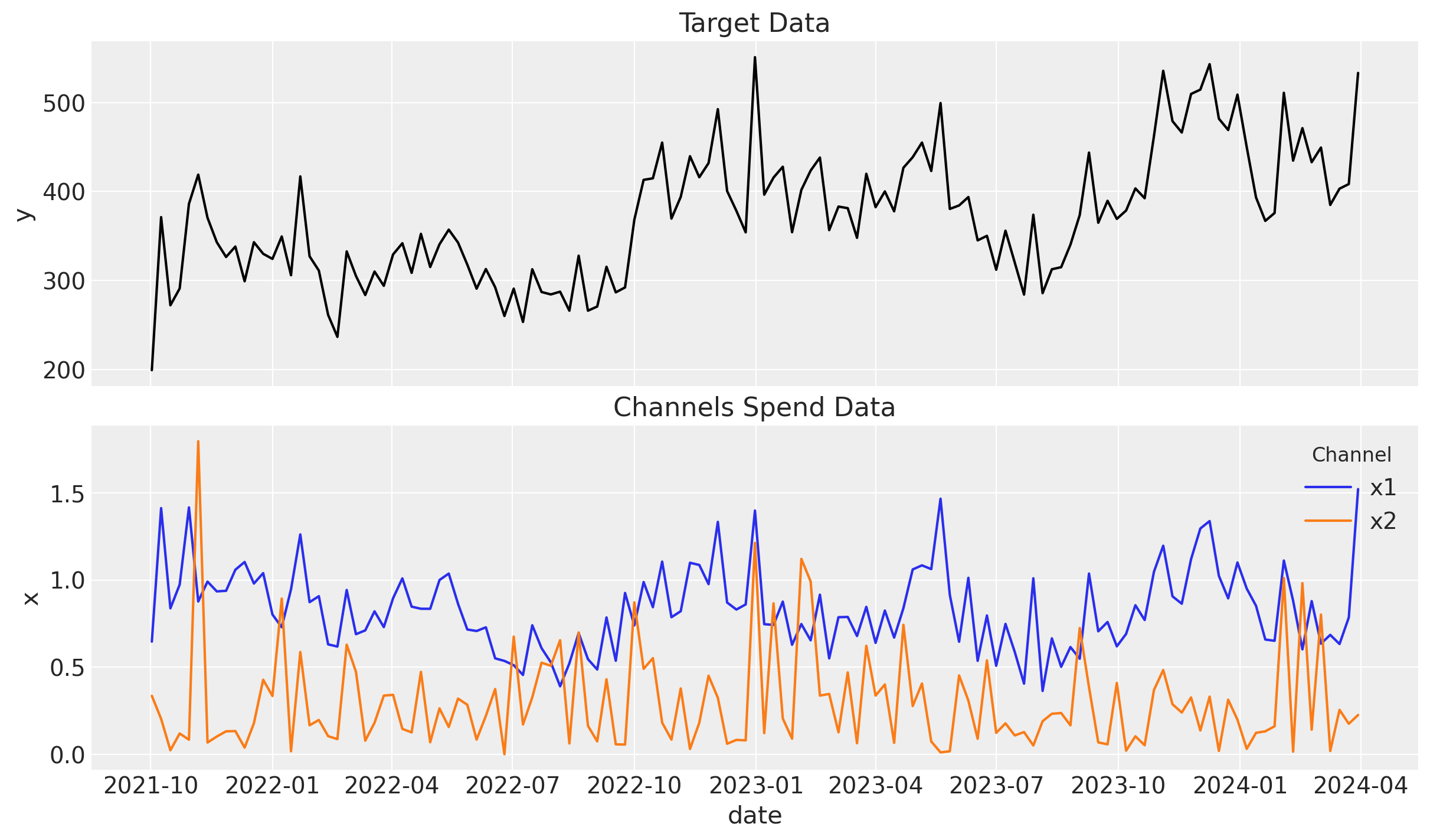
Before jumping into the model, let’s plot the target data and the channels data to understand it better.

fig, ax = plt.subplots(
    nrows=2,
    ncols=1,
    sharex=True,
    sharey=False,
    layout="constrained",
)

sns.lineplot(
    x="date",
    y="y",
    data=model_df,
    color="black",
    ax=ax[0],
)
ax[0].set_title("Target Data")

model_df.melt(
    id_vars=["date"], value_vars=["x1", "x2"], var_name="channel", value_name="x"
).pipe(
    (sns.lineplot, "data"),
    x="date",
    y="x",
    hue="channel",
    ax=ax[1],
)
ax[1].legend(title="Channel", title_fontsize=12)
ax[1].set_title("Channels Spend Data");

../../_images/52c11837155fa55139f0b9eee3f7d93ed3510f8c04107b3fccefe0a13da82370.png

Baseline Model#

To begin with, we fit a media mix model, without including the unobserved confounder z, using a geometric adstock and logistic saturation using PyMC-Marketing’s API. For more details on the model, please refer to the MMM Example Notebook notebook. As we discuss in that notebook, without any lift test information, a good starting point is to pass the cost share into the prior of the beta channel coefficients.

cost_share = DataArray(
    model_df[["x1", "x2"]].sum() / model_df[["x1", "x2"]].sum().sum(),
    dims="channel",
)

We can specify the model configuration as follows (see the Model Configuration notebook for more details):

model_config = {
    "likelihood": Prior("Normal", sigma=Prior("HalfNormal", sigma=2)),
    "gamma_fourier": Prior("Normal", mu=0, sigma=2, dims="fourier_mode"),
    "intercept_tvp_config": HSGPKwargs(
        m=100, L=None, eta_lam=1.0, ls_mu=5.0, ls_sigma=10.0, cov_func=None
    ),
    "adstock_alpha": Prior("Beta", alpha=2, beta=3, dims="channel"),
    "saturation_lam": Prior("Gamma", alpha=2, beta=2, dims="channel"),
    "saturation_beta": Prior("HalfNormal", sigma=cost_share, dims="channel"),
}

Observe that we are going to use a Gaussian process to model the non-linear trend component (see MMM with time-varying parameters (TVP)).

Let’s fit the model!

%%time

mmm = MMM(
    adstock=GeometricAdstock(l_max=4),
    saturation=LogisticSaturation(),
    date_column="date",
    channel_columns=["x1", "x2"],
    target_column="y",
    time_varying_intercept=True,
    time_varying_media=False,
    yearly_seasonality=5,
    model_config=model_config,
)

y = model_df["y"]
X = model_df.drop(columns=["y"])

sampler_config = {
    "tune": 1_000,
    "chains": 4,
    "draws": 1_000,
    "nuts_sampler": "nutpie",
    "target_accept": 0.95,
    "random_seed": rng,
}

mmm.build_model(X, y)
mmm.add_original_scale_contribution_variable(
    var=[
        "channel_contribution",
        "fourier_contribution",
        "intercept_contribution",
    ]
)
_ = mmm.fit(X, y, **sampler_config)
_ = mmm.sample_posterior_predictive(
    X, extend_idata=True, combined=True, random_seed=rng
)

Sampler Progress

Total Chains: 4

Active Chains: 0

Finished Chains: 4

Sampling for 12 seconds

Estimated Time to Completion: now

Draws	Divergences	Step Size	Gradients/Draw
2000	0	0.08	63
2000	0	0.09	63
2000	1	0.10	127
2000	0	0.08	63

Sampling: [y]

CPU times: user 59 s, sys: 1.19 s, total: 1min
Wall time: 24.6 s

Let’s verify that we do not have divergent transitions.

# Number of diverging samples
mmm.idata["sample_stats"]["diverging"].sum().item()

../../_images/8ff45515122bf7560362e527c8ac20126ffbf8eae3a51b1eecff38c64abffa7b.png

Next, we look into the model components contributions:

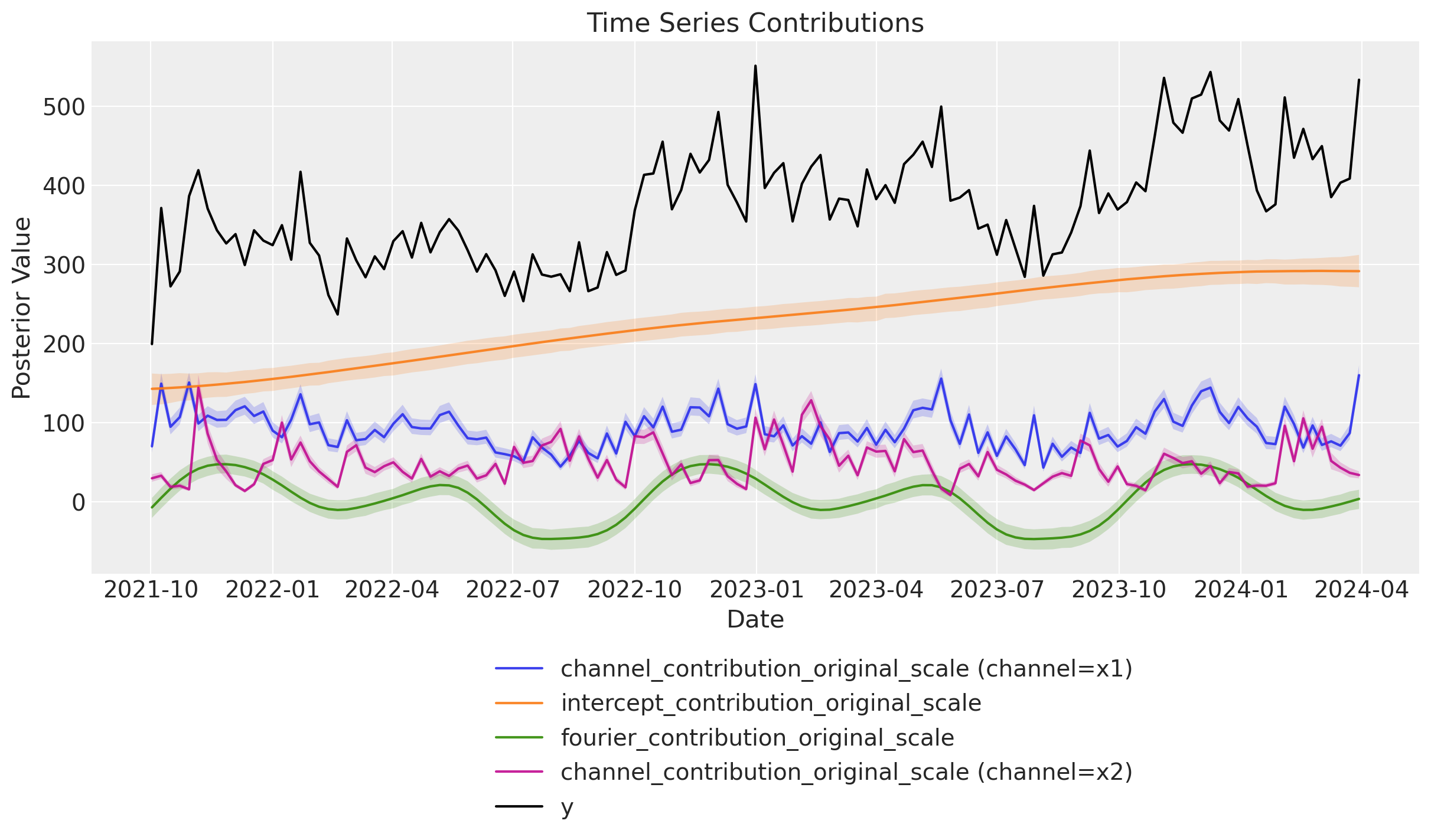
fig, axes = mmm.plot.contributions_over_time(
    var=[
        "channel_contribution_original_scale",
        "intercept_contribution_original_scale",
        "fourier_contribution_original_scale",
    ],
    dims={"channel": ["x1", "x2"]},
    combine_dims=True,
    hdi_prob=0.94,
    figsize=(12, 7),
)
sns.lineplot(x="date", y="y", data=model_df, color="black", label="y", ax=axes[0, 0])
legend = axes[0, 0].get_legend()
legend.set_bbox_to_anchor((0.8, -0.12))

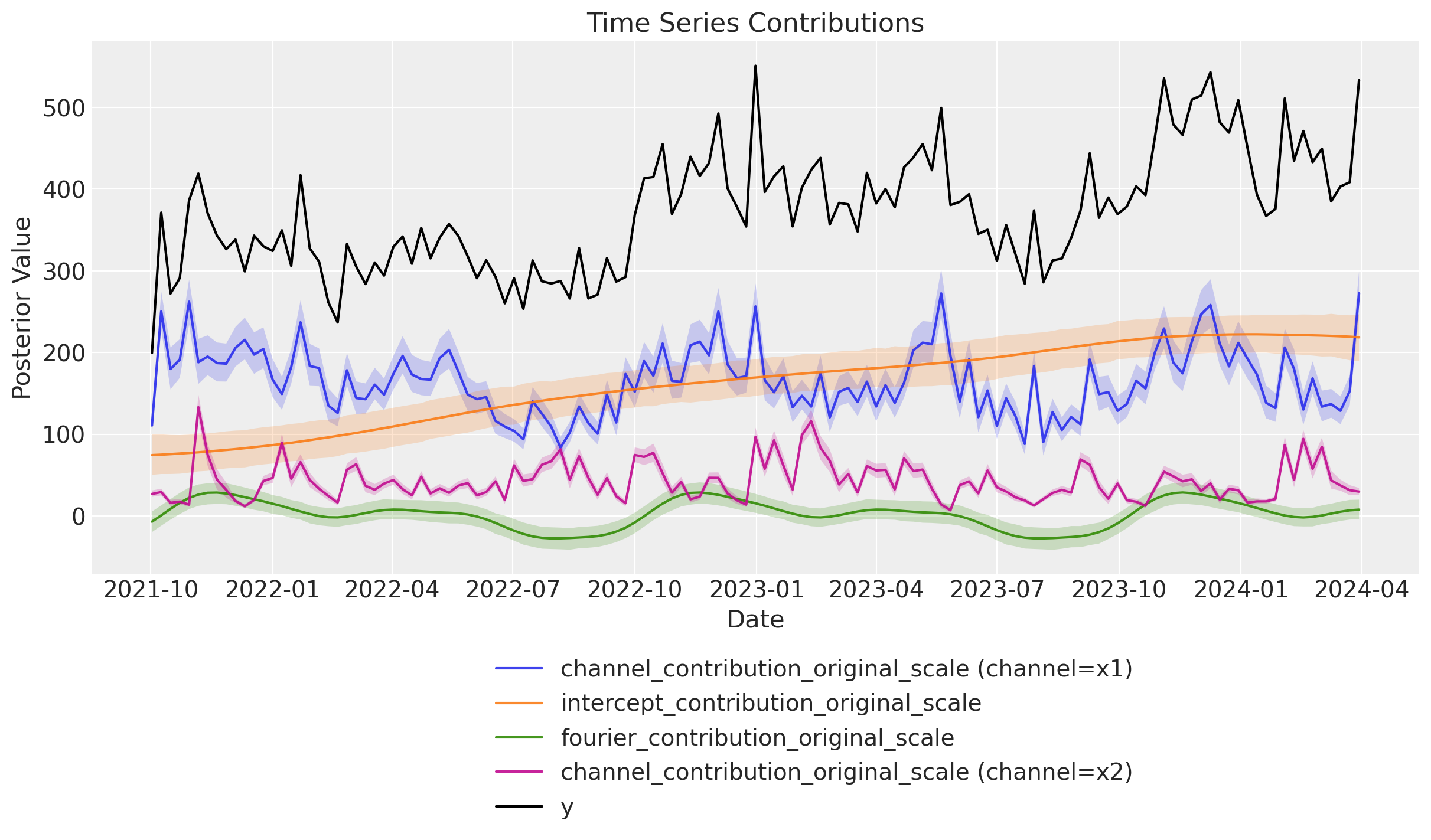
../../_images/a51943aaa49e6b3d5afaa99a55da3f8d6253764de814b898285135930c903161.png

The results look very similar to the results from the original blog post. In particular, note that we were able to capture the non-linear trend.

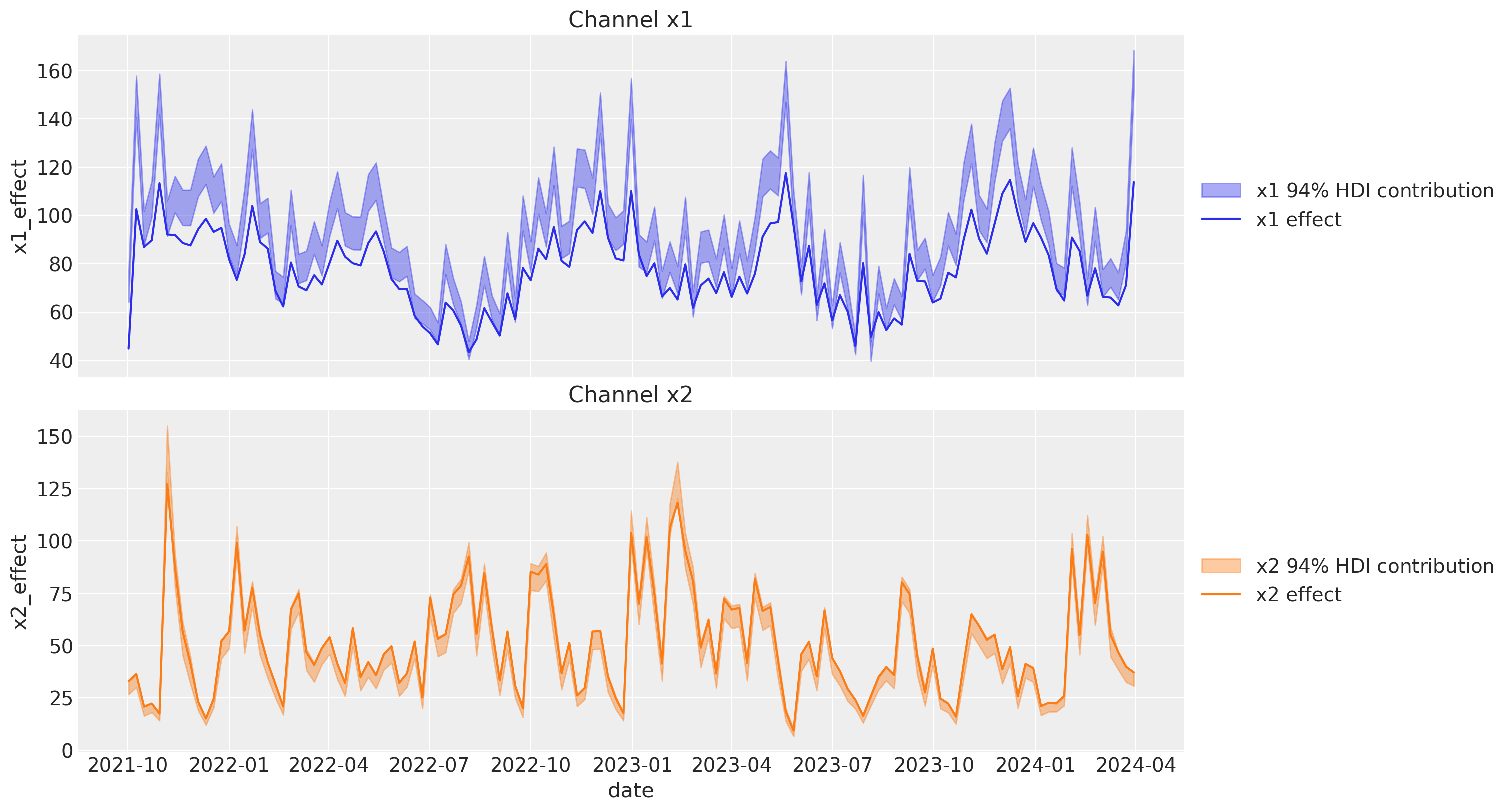
Next, we look into the channel contributions against the true effects (which we know from the data generating process).

channels_contribution_original_scale = mmm.idata["posterior"][
    "channel_contribution_original_scale"
]
channels_contribution_original_scale_hdi = az.hdi(
    ary=channels_contribution_original_scale
)

fig, ax = plt.subplots(
    nrows=2, figsize=(15, 8), ncols=1, sharex=True, sharey=False, layout="constrained"
)

amplitude = 100

for i, x in enumerate(["x1", "x2"]):
    # HDI estimated contribution in the original scale
    ax[i].fill_between(
        x=model_df["date"],
        y1=channels_contribution_original_scale_hdi[
            "channel_contribution_original_scale"
        ].sel(channel=x, hdi="lower"),
        y2=channels_contribution_original_scale_hdi[
            "channel_contribution_original_scale"
        ].sel(channel=x, hdi="higher"),
        color=f"C{i}",
        label=rf"{x} $94\%$ HDI contribution",
        alpha=0.4,
    )
    sns.lineplot(
        x="date",
        y=f"{x}_effect",
        data=raw_df.assign(**{f"{x}_effect": lambda df: amplitude * df[f"{x}_effect"]}),  # noqa B023
        color=f"C{i}",
        label=f"{x} effect",
        ax=ax[i],
    )

    ax[i].legend(loc="center left", bbox_to_anchor=(1, 0.5))
    ax[i].set(title=f"Channel {x}")

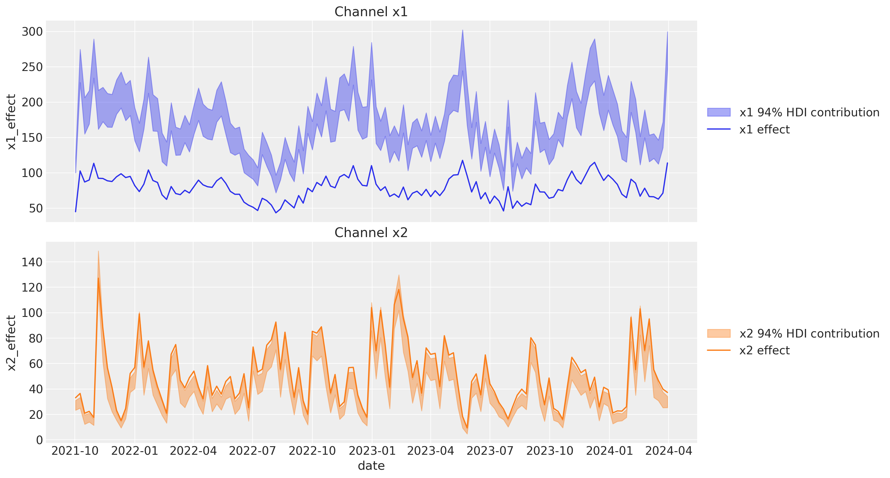
../../_images/2d255d2c2d910e14b68e648ec3dd4e1304913fd7a800e065e927df491c96acd2.png

We see that the contribution for x1 is very different from the true effect. This is because the absence of the unobserved confounder z. For x2, the contribution is very similar to the true effect.

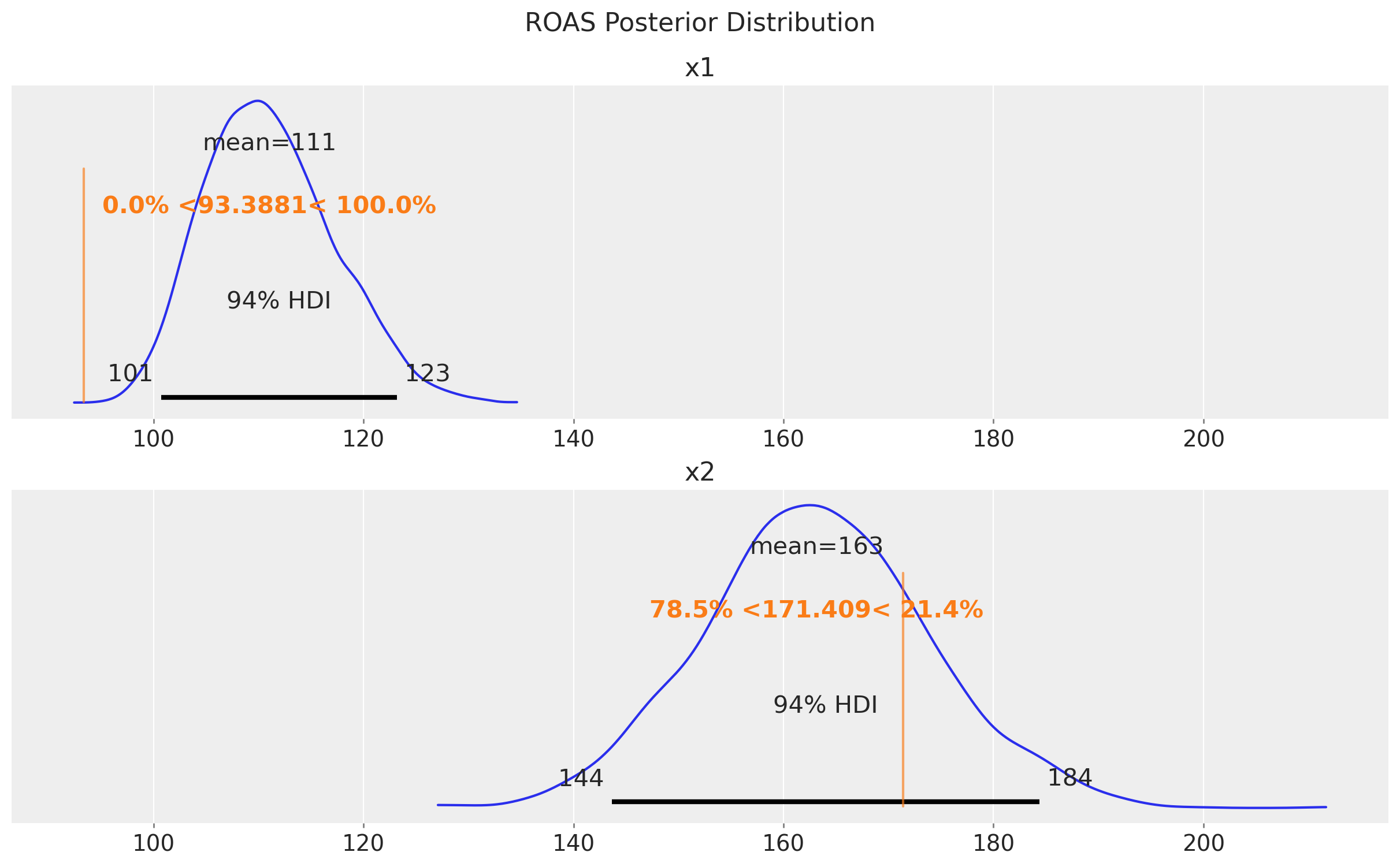
Finally, we can compute the ROAS for the x1 and x2 channels (again, ignoring the small carryover effect).

roas_posterior = mmm.incrementality.contribution_over_spend(
    frequency="all_time"
).rename("roas")

fig, ax = plt.subplots(
    nrows=2, ncols=1, figsize=(12, 7), sharex=True, sharey=False, layout="constrained"
)

az.plot_posterior(roas_posterior, ref_val=[true_roas_x1, true_roas_x2], ax=ax)
ax[0].set_title("x1")
ax[1].set_title("x2")
fig.suptitle("ROAS Posterior Distribution", fontsize=16, y=1.05);

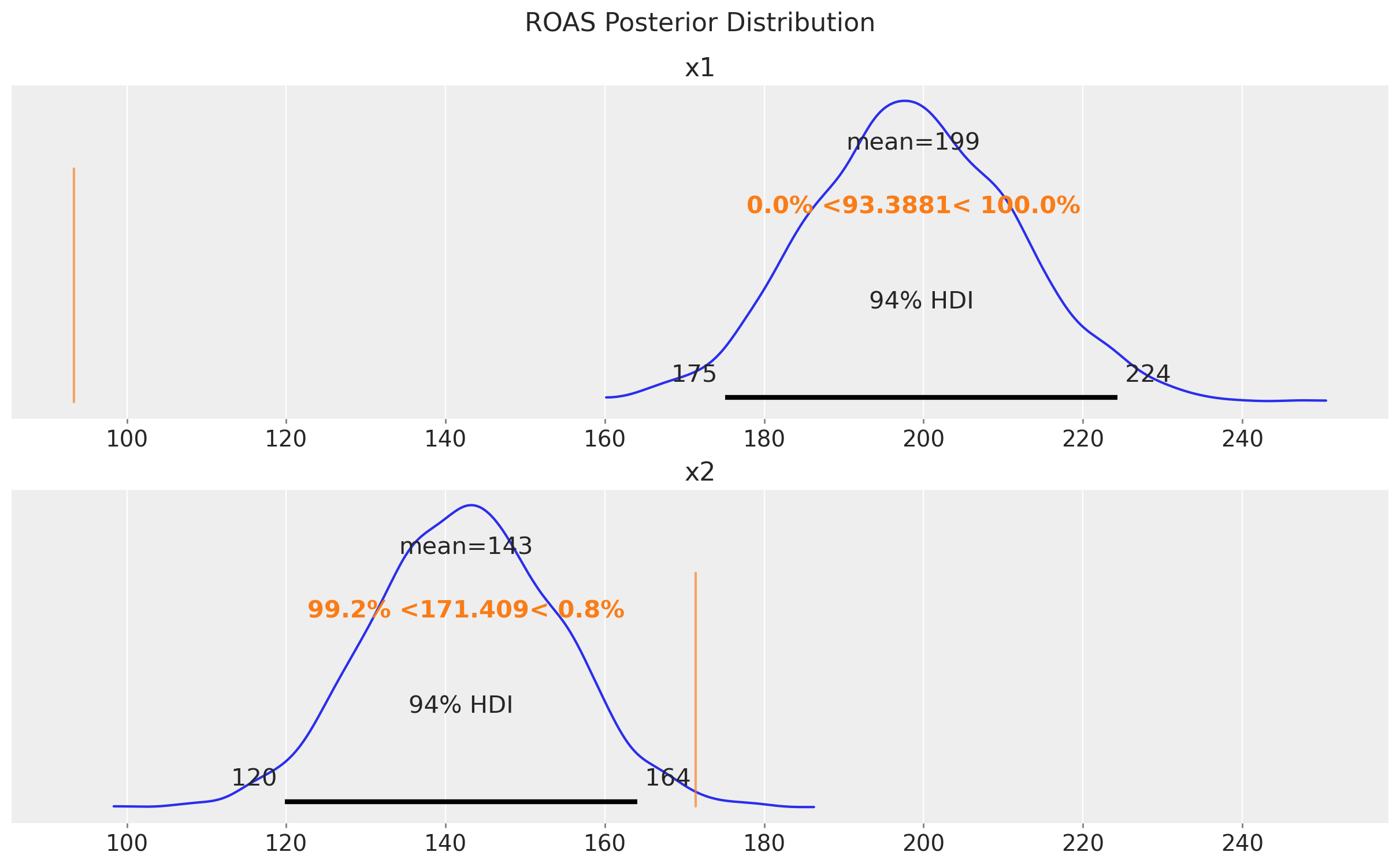
../../_images/9abe26de531684d10e9185e67ef4102711ed495a1978a2d81e39e6ad5a326bf6.png

We see that the ROAS for x1 is very different from the true value. This is reflecting the bias induced by the unobserved confounder z. The models suggests that x1 is more effective than x2, but we know from the data generating process that x2 is more effective!

Lift Test Model#

Now we fit a model with some lift tests. We will use the same model configuration as before, but we free the priors of the beta channel coefficients as these are included in the saturation function parametrization. In general, we expect lift test priors or associated custom likelihoods to be better than the cost share prior.

model_config = {
    "likelihood": Prior("Normal", sigma=Prior("HalfNormal", sigma=2)),
    "gamma_fourier": Prior("Normal", mu=0, sigma=2, dims="fourier_mode"),
    "intercept_tvp_config": HSGPKwargs(
        m=50, L=None, eta_lam=1.0, ls_mu=5.0, ls_sigma=10.0, cov_func=None
    ),
    "adstock_alpha": Prior("Beta", alpha=2, beta=3, dims="channel"),
    "saturation_lam": Prior("Gamma", alpha=2, beta=2, dims="channel"),
    "saturation_beta": Prior("HalfNormal", sigma=cost_share, dims="channel"),
}

mmm_lift = MMM(
    adstock=GeometricAdstock(l_max=4),
    saturation=LogisticSaturation(),
    date_column="date",
    channel_columns=["x1", "x2"],
    target_column="y",
    time_varying_intercept=True,
    time_varying_media=False,
    yearly_seasonality=5,
    model_config=model_config,
)

# we need to build the model before adding the lift test measurements
mmm_lift.build_model(X, y)

Lift Tests

In a lift study, one temporarily changes the budget of a channel for a fixed period of time, and then uses some method (for example CausalPy) to make inference about the change in sales directly caused by the adjustment.

A lift test is characterized by:

channel: the channel that was tested
x: pre-test channel spend
delta_x: change made to x
delta_y: inferred change in sales due to delta_x
sigma: standard deviation of delta_y

An experiment characterized in this way can be viewed as two points on the saturation curve for the channel.

Next assume we have ran two lift tests for the x1 and x2 channels. The results table looks like this:

df_lift_test = pd.DataFrame(
    data={
        "channel": ["x1", "x2", "x1", "x2"],
        "x": [0.25, 0.1, 0.8, 0.25],
        "delta_x": [0.25, 0.1, 0.8, 0.25],
        "delta_y": [
            true_roas_x1 * 0.25,
            true_roas_x2 * 0.1,
            true_roas_x1 * 0.8,
            true_roas_x2 * 0.25,
        ],
        "sigma": [3, 3, 3, 3],
        "date": pd.to_datetime(
            [
                X["date"].max() - pd.Timedelta(weeks=50),
                X["date"].max() - pd.Timedelta(weeks=30),
                X["date"].max() - pd.Timedelta(weeks=14),
                X["date"].max() - pd.Timedelta(weeks=12),
            ]
        ),
    }
)

df_lift_test

	channel	x	delta_x	delta_y	sigma	date
0	x1	0.25	0.25	23.347033	3	2023-04-15
1	x2	0.10	0.10	17.140880	3	2023-09-02
2	x1	0.80	0.80	74.710505	3	2023-12-23
3	x2	0.25	0.25	42.852201	3	2024-01-06

Comparison with the original blog post

Note that we have added the true ROAS for the x1 and x2 channels implicit to the df_lift_test table. We add them by multiplying the delta_y as this is what we would have observed if we had run the lift test (or similar values).

In the simulation Media Mix Model and Experimental Calibration: A Simulation Study, the author included these “true” values into the prior for the ROAS.

Now, we fit the model with the lift test measurements.

mmm_lift.add_lift_test_measurements(df_lift_test=df_lift_test)

<pymc_marketing.mmm.mmm.MMM at 0x3206a6ff0>

mmm_lift.add_original_scale_contribution_variable(
    var=[
        "channel_contribution",
        "fourier_contribution",
        "intercept_contribution",
    ]
)
_ = mmm_lift.fit(X, y, **sampler_config)
_ = mmm_lift.sample_posterior_predictive(
    X, extend_idata=True, combined=True, random_seed=rng
)

Sampler Progress

Total Chains: 4

Active Chains: 0

Finished Chains: 4

Sampling for now

Estimated Time to Completion: now

Draws	Divergences	Step Size	Gradients/Draw
2000	0	0.09	63
2000	0	0.10	95
2000	1	0.09	63
2000	0	0.10	95

Sampling: [lift_measurements, y]

Again, we verify that we do not have divergent transitions.

# Number of diverging samples
mmm_lift.idata["sample_stats"]["diverging"].sum().item()

Let’s plot the components contributions as we did before.

fig, axes = mmm_lift.plot.contributions_over_time(
    var=[
        "channel_contribution_original_scale",
        "intercept_contribution_original_scale",
        "fourier_contribution_original_scale",
    ],
    dims={"channel": ["x1", "x2"]},
    combine_dims=True,
    hdi_prob=0.94,
    figsize=(12, 7),
)
sns.lineplot(x="date", y="y", data=model_df, color="black", label="y", ax=axes[0, 0])
legend = axes[0, 0].get_legend()
legend.set_bbox_to_anchor((0.8, -0.12))

../../_images/059775e208e42a6b3fc0486f3298b993f544bc6b139b762f5e89c61affcec2af.png

As before, we have recovered the non-linear trend component and the yearly seasonality.

Now, let’s compare the channel contributions to the true ones.

channels_contribution_original_scale = mmm_lift.idata["posterior"][
    "channel_contribution_original_scale"
]
channels_contribution_original_scale_hdi = az.hdi(
    ary=channels_contribution_original_scale, hdi_prob=0.8
)

fig, ax = plt.subplots(
    nrows=2, figsize=(15, 8), ncols=1, sharex=True, sharey=False, layout="constrained"
)

amplitude = 100

for i, x in enumerate(["x1", "x2"]):
    # HDI estimated contribution in the original scale
    ax[i].fill_between(
        x=model_df["date"],
        y1=channels_contribution_original_scale_hdi[
            "channel_contribution_original_scale"
        ].sel(channel=x, hdi="lower"),
        y2=channels_contribution_original_scale_hdi[
            "channel_contribution_original_scale"
        ].sel(channel=x, hdi="higher"),
        color=f"C{i}",
        label=rf"{x} $94\%$ HDI contribution",
        alpha=0.4,
    )
    sns.lineplot(
        x="date",
        y=f"{x}_effect",
        data=raw_df.assign(**{f"{x}_effect": lambda df: amplitude * df[f"{x}_effect"]}),  # noqa B023
        color=f"C{i}",
        label=f"{x} effect",
        ax=ax[i],
    )

    ax[i].legend(loc="center left", bbox_to_anchor=(1, 0.5))
    ax[i].set(title=f"Channel {x}")

../../_images/513d31b8b6a33e737b7202d57f28cfd684a63fc130c5d686fc7cc7347d6d5627.png

The contributions look much better and they are very close to the ones of the original blog post! Hence, these two approaches are very similar. However note that the PyMC-Marketing approach is more flexible as it allows us to enrich the estimates with more tests and different media spends to have a better understanding of the saturation effect.

Finally, let’s compute the ROAS for the x1 and x2 channels.

roas_posterior = mmm_lift.incrementality.contribution_over_spend(
    frequency="all_time"
).rename("roas")

fig, ax = plt.subplots(
    nrows=2, ncols=1, figsize=(12, 7), sharex=True, sharey=False, layout="constrained"
)

az.plot_posterior(roas_posterior, ref_val=[true_roas_x1, true_roas_x2], ax=ax)
ax[0].set_title("x1")
ax[1].set_title("x2")
fig.suptitle("ROAS Posterior Distribution", fontsize=16, y=1.05);

../../_images/0927de3e86a431b3e9aa2ed22b015153bb85169827e54cfa9299bb89604936c5.png

The estimates are very very close to the true ROAS! We do get from the model that x2 is more effective than x1, which is aligned with the lift test results!

Note

For this specific simulation, the results are better than the ones of the original simulation study Media Mix Model and Experimental Calibration: A Simulation Study where the ROAS paramtrization is employed. Why? As we will see in the next section, we can leverage the on different spend levels to have a better understanding of the saturation effect and therefore improve the estimates.

Time Slice Cross Validation#

We have seen how two similar models can provide different ROAS estimates. To better understand the stability of the estimates, we can perform a time slice cross validation as described in the example notebook Time-Slice-Cross-Validation and Parameter Stability.

We illustrate the procedure below. Observe that for the calibrated model, we can pass the lift test measurements to the df_lift_test argument. The cross-validation implementation ensures we do not leak any information by preventing tests from being used for fitting if they are after the end of the training data.

%%time

cv = TimeSliceCrossValidator(
    n_init=115,
    forecast_horizon=12,
    date_column="date",
    step_size=1,
)


cv_results, mmms = cv.run(
    X=X,
    y=y,
    mmm=mmm,
    original_scale_vars=["channel_contribution", "y"],
    sampler_config=sampler_config | {"progressbar": False},
    return_models=True,
)

cv_results_lift, mmms_lift = cv.run(
    X=X,
    y=y,
    mmm=mmm_lift,
    df_lift_test=df_lift_test,
    lift_test_date_column="date",
    original_scale_vars=["channel_contribution", "y"],
    sampler_config=sampler_config | {"progressbar": False},
    return_models=True,
)

Sampling: [y]

Sampling: [y]

Sampling: [y]

Sampling: [y]

Sampling: [y]

Sampling: [lift_measurements, y]

Sampling: [lift_measurements, y]

Sampling: [lift_measurements, y]

Sampling: [lift_measurements, y]

Sampling: [lift_measurements, y]

CPU times: user 9min 8s, sys: 14.4 s, total: 9min 23s
Wall time: 4min 7s

Parameter Development over Folds#

Let’s start by looking into how the parameters develop over the folds for both models. We are interested in assesing if they change significantly and if so, understand the reason behind it.

# Baseline model
fig, ax = cv.plot.param_stability(
    cv_data=cv_results, var_names=["saturation_beta"], figsize=(10, 6)
)
fig.suptitle(
    "Saturation Beta over Folds - Baseline Model",
    fontsize=18,
    fontweight="bold",
    y=1.06,
)

# Calibrated model
fig, ax = cv.plot.param_stability(
    cv_data=cv_results_lift, var_names=["saturation_beta"], figsize=(10, 6)
)
fig.suptitle(
    "Saturation Beta over Folds - Calibrated Model",
    fontsize=18,
    fontweight="bold",
    y=1.06,
);

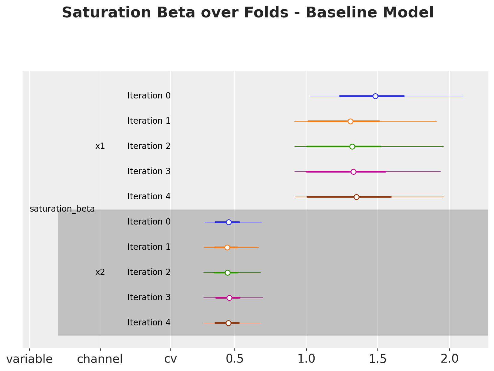
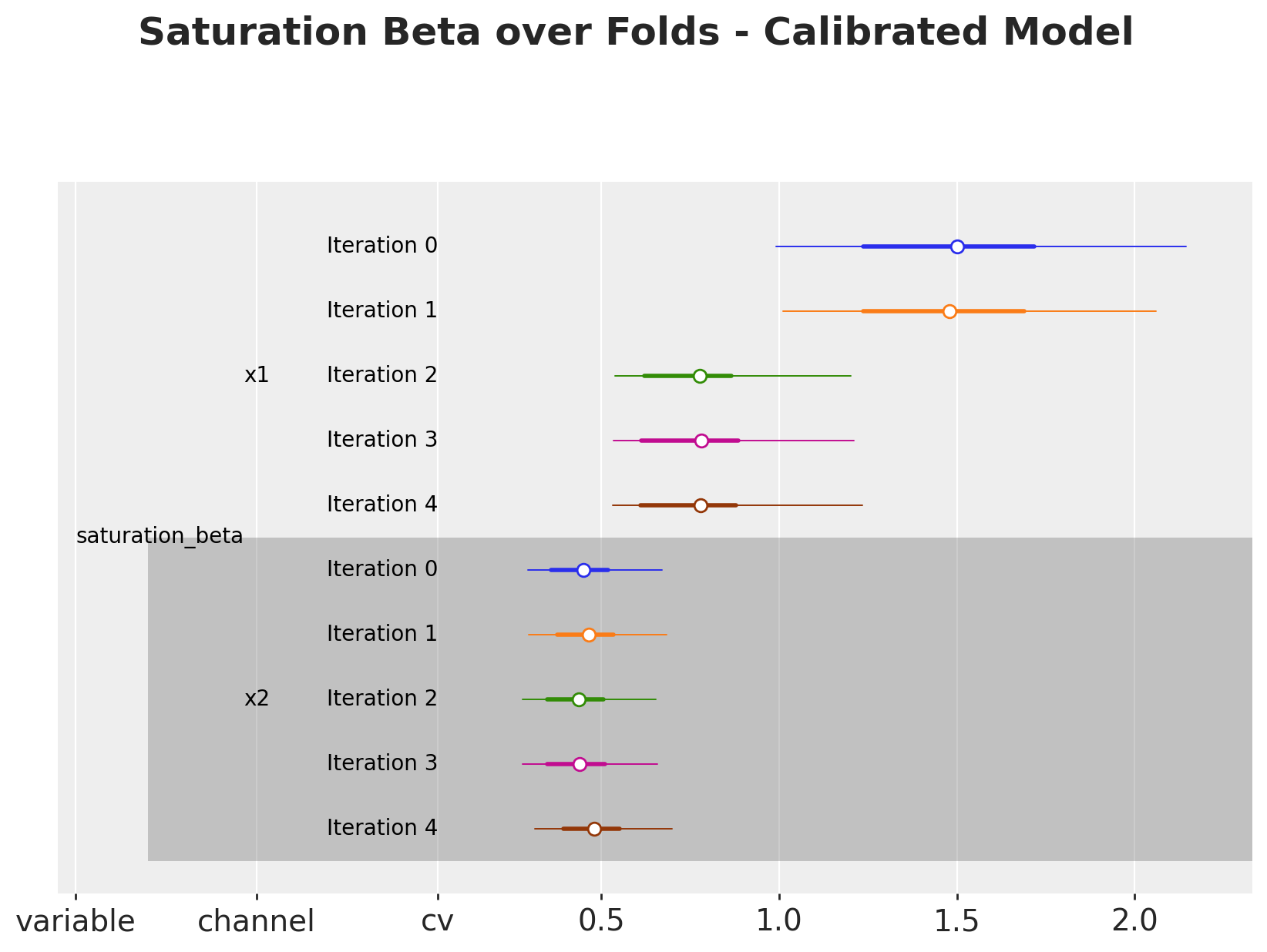
../../_images/3f5e57f9ba913538c6f8d1e465923dc48044a99e9121791c2015825041682e26.png

../../_images/7be8ea946b411981b4d42fb49fe5a857c00f10e60741050a0ebd47b11ea172b5.png

Overall, the parameters are very stable for the baseline model (top plot). For the calibrated model (bottom plot), we see that for channel x1, the parameters shift after the third iteration. This is because we have some experiments which are being added into the training data as the folds move. This shows the lift test calibration in action!

Let’s look into the experiment dates and the fold boundaries to make this more concrete.

fig, ax = plt.subplots()
sns.lineplot(x="date", y="y", data=model_df, color="black", label="y", ax=ax)


for fold_idx in range(len(cv_results["cv_metadata"]["metadata"])):
    start_date_test_fold = (
        cv_results["cv_metadata"]["metadata"]
        .sel(cv=f"Iteration {fold_idx}")
        .values.item()["X_test"]["date"]
        .min()
    )
    ax.axvline(start_date_test_fold, color="gray", linestyle="--")

for row in df_lift_test.itertuples():
    color = "C0" if row.channel == "x1" else "C1"
    ax.axvline(row.date, color=color, linestyle="--")

ax.legend()
ax.set_title(
    "Lift Test Measurements and Fold Boundaries", fontsize=18, fontweight="bold"
);

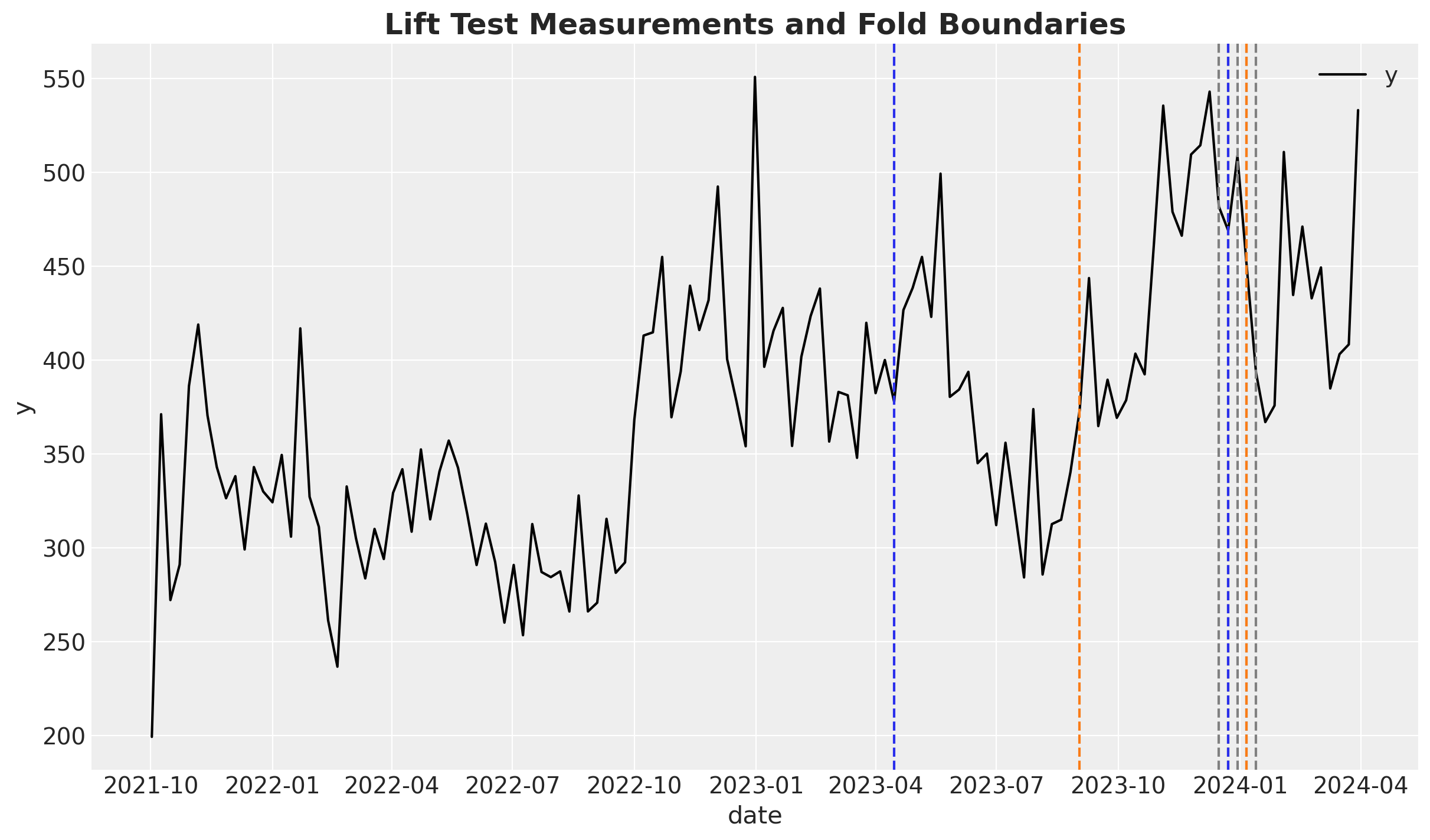
../../_images/620991d8c0826b28f98c55a920fa86a151ac25f78b23379fd044a37f3709baf7.png

Here we see the target variable in black and the fold boundaries in gray. The lift test measurements are in dashed lines (blue for x1 and red for x2). We see that some lift tests are added into the training data as the folds move. This is the key explanation of the parameter fluctuation over folds for channel x1 in the calibrated model. The more experiments we add to the training data, the more accurate (causaly speaking) the model is.

We can continue the analysis by looking into the lambda parameters, which have a direct interpretation as the saturation effect.

# Baseline model
fig, ax = cv.plot.param_stability(
    cv_data=cv_results, var_names=["saturation_lam"], figsize=(10, 6)
)
fig.suptitle(
    "Saturation Lambda over Folds - Baseline Model",
    fontsize=18,
    fontweight="bold",
    y=1.06,
)

# Calibrated model
fig, ax = cv.plot.param_stability(
    cv_data=cv_results_lift, var_names=["saturation_lam"], figsize=(10, 6)
)
fig.suptitle(
    "Saturation Lambda over Folds - Calibrated Model",
    fontsize=18,
    fontweight="bold",
    y=1.06,
);

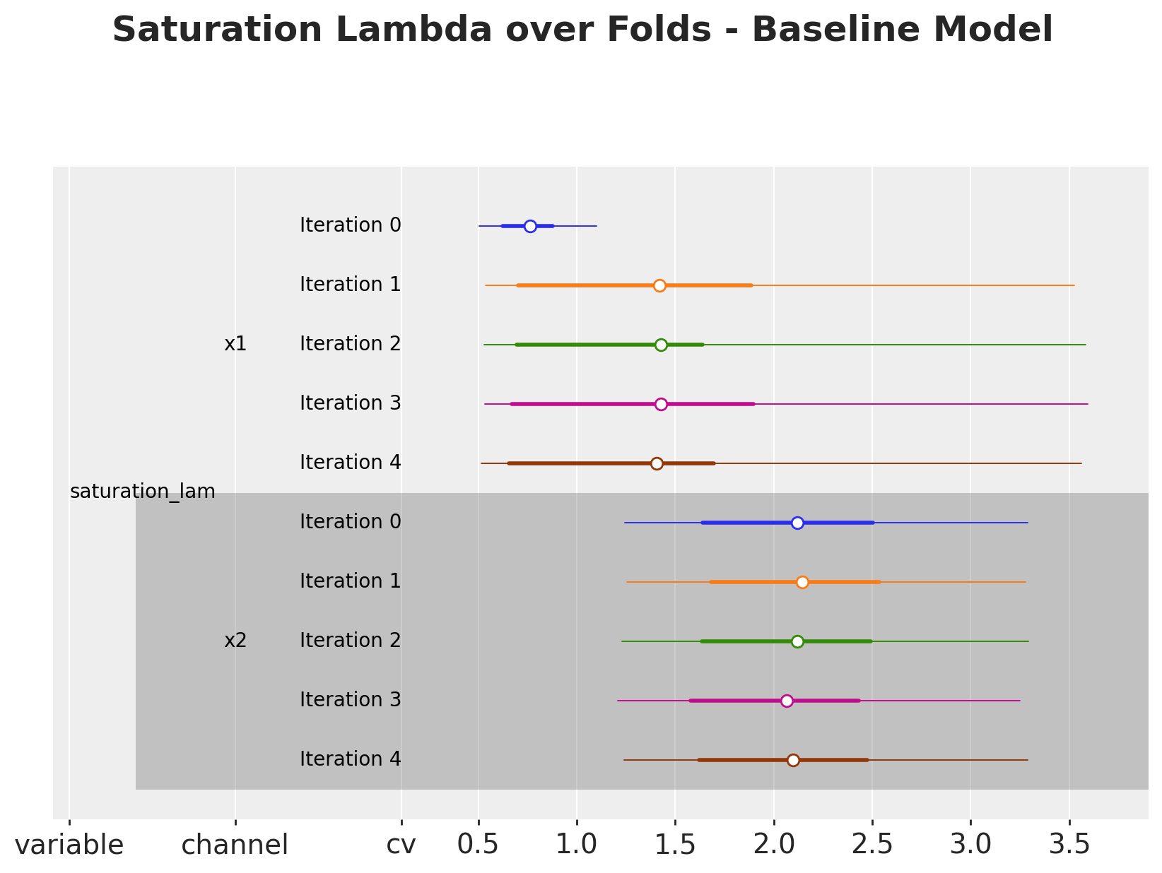
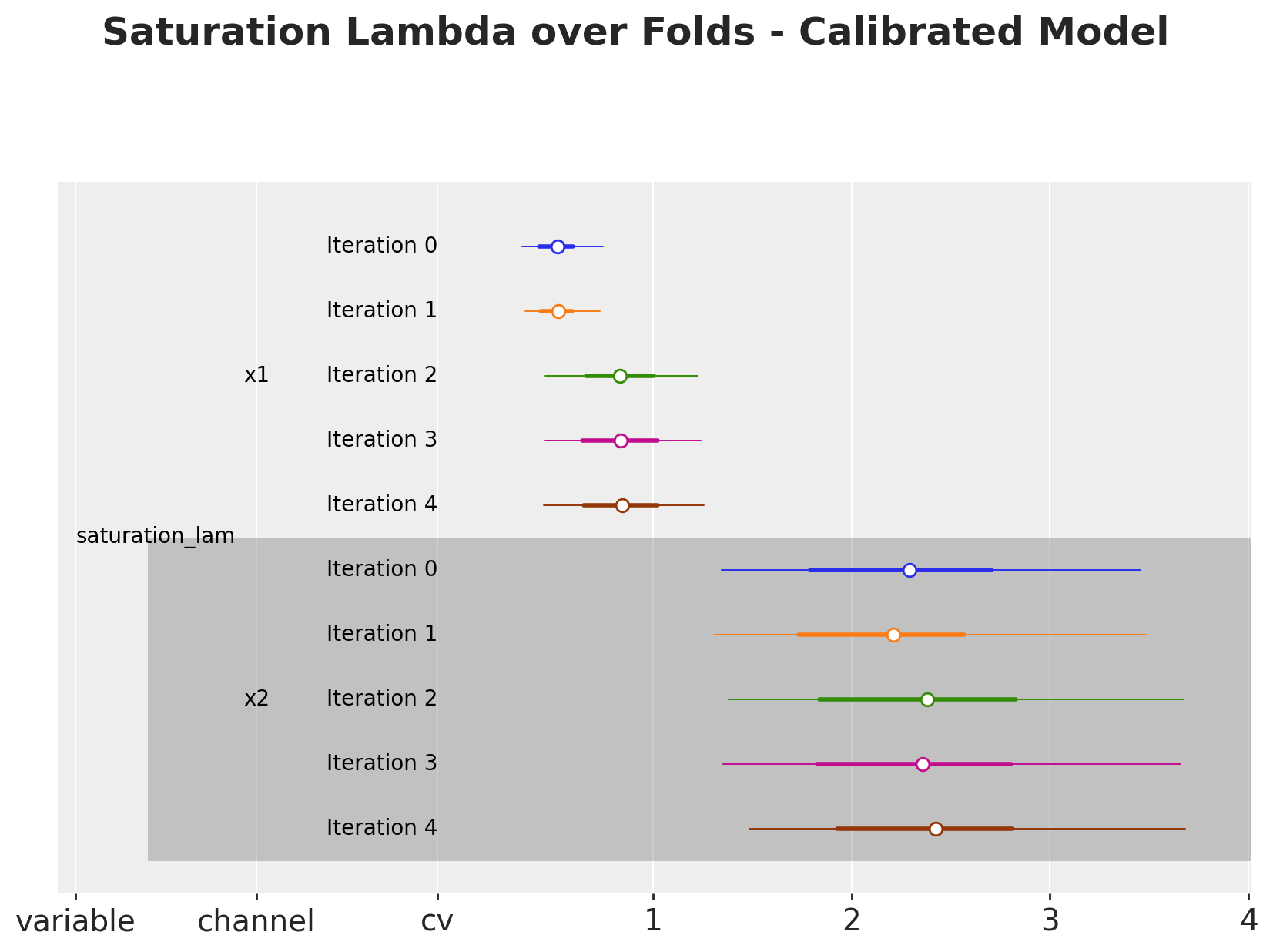
../../_images/ce302a75081deb3c699103843506ac9cd32bdd4cf749418ccaeadf37b022a7bc.png

../../_images/516d3782b1888d62311f061282819a264039f79cf268a2a9a5f703e1e016dd09.png

As expected, the lambda are also affected by the lift test calibration as we add more tests.

Now we look into a metric of interest: the ROAS. The following code just computes the ROAS for each fold.

def get_fold_roas(models: list[MMM], fold_idx: int) -> DataArray:
    return (
        models[fold_idx]
        .incrementality.contribution_over_spend(frequency="all_time")
        .rename("roas")
    )


fold_roas = [get_fold_roas(mmms, i) for i in range(len(mmms))]

fold_roas_lift = [get_fold_roas(mmms_lift, i) for i in range(len(mmms_lift))]

Let’s visualize the results

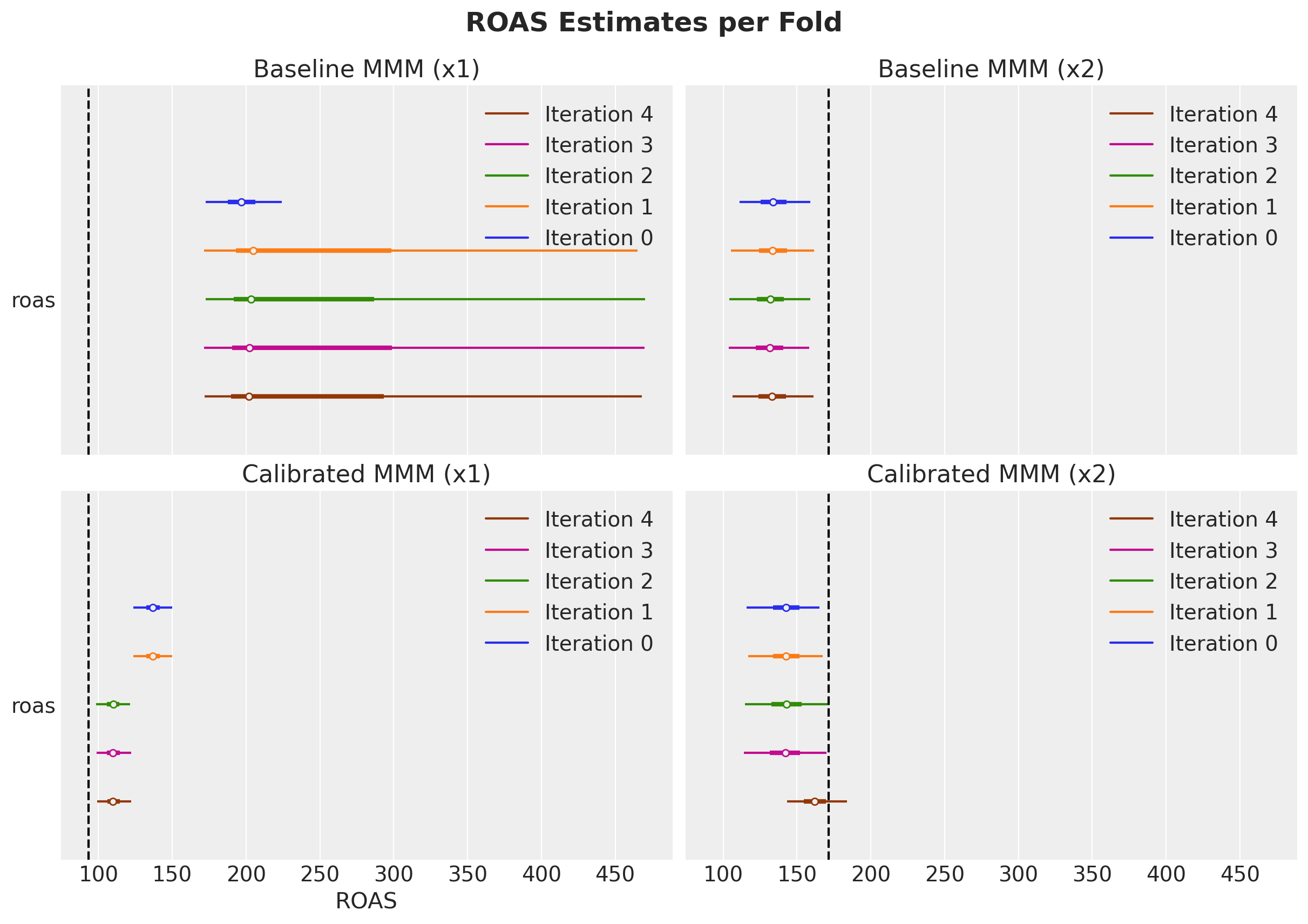
../../_images/279279c12fde33ac7fe6ae0249b74e209c0166e6423109a8752ff38087609d97.png

The bottom plot, corresponding to the calibrated model, shows that as we add more lift test measurements, the ROAS estimates stabilize and converge to the true ROAS 🚀!

Tip

This shows the power of a joint measurement strategy between experimentation and marketing mix modelling.

Out-of-sample Predictions#

Finally, we cant to look into the out-of-sample predictions of the models for each fold. To quantify the performance of the models, we consider the Continuous Ranked Probability Score (CRPS). This metric is a generalization of the mean absolute error (MAE) to the probabilistic predictions setting. Intuitively, the CRPS measures the “distance” between the predicted distribution and the observed value by comparing their cummulative distribution function (CDF) at every point on the real line. For more details, take a look into the blog post “Intuition behind CRPS”.

Let’s compute the CRPS for each fold and visualize the results.

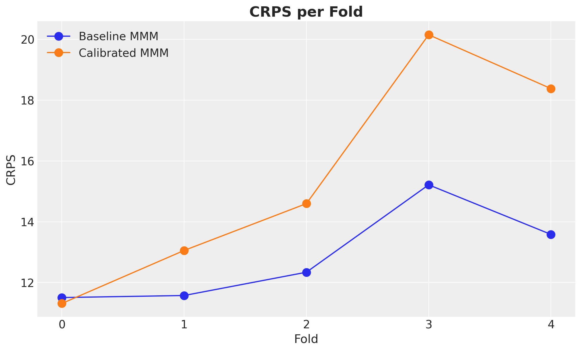
../../_images/e9b526b8983007523488bf7ef934f7bb8adf2889c264e18259e87779e6ed3b35.png

The baseline model consistently outperforms the calibrated model with respect to the CRPS on the test set. This illustrates a key point about marketing mix models: out-of-sample performance is not the only metric to validate a model. It is a good metric, but it is not the only one. We need to validate the model through experiments (interventions) as this inherently a causal inference problem.

Conclusion#

In this notebook, we have seen a concrete example of how media mix models can provide biased estimates when we have unobserved confounders in the model specification. Ideally, we’d add the confounder, but in the absence of that, we need to provide a reality anchor to the model to have meaningful estimates. We have shown that the PyMC-Marketing approach of adding lift test measurements to the model is very similar to the one proposed in the paper Media Mix Model Calibration With Bayesian Priors and the blog post Media Mix Model and Experimental Calibration: A Simulation Study.

However, the PyMC-Marketing approach is more flexible as it allows enriching the estimates with more lift tests and different media spending to better understand the saturation effect. We explicitly see this phenomenon by performing a time slice cross validation analysis and observing how the ROAS estimates stabilize and approach the true ROAS as more lift tests are added.

%load_ext watermark
%watermark -n -u -v -iv -w

Last updated: Fri, 01 May 2026

Python implementation: CPython
Python version       : 3.12.13
IPython version      : 9.12.0

arviz         : 0.23.4
graphviz      : 0.21
matplotlib    : 3.10.8
numpy         : 2.4.3
pandas        : 2.3.3
pymc_extras   : 0.10.0
pymc_marketing: 0.19.2
seaborn       : 0.13.2
xarray        : 2026.2.0

Watermark: 2.6.0