Consideration Set Mixed Logit: Separating Attention from Preference

This notebook demonstrates a two-stage discrete choice model that separates which alternatives get considered from which is preferred. We apply it to the Swiss Metro stated-preference dataset (Train, SwissMetro, Car), compare a vanilla model with one that adds random effects on travel time, and show that the consideration-stage estimates can change dramatically when the utility stage is better specified.

import warnings

import arviz as az
import matplotlib.pyplot as plt
import numpy as np
import pandas as pd
import pymc as pm

from pymc_marketing.customer_choice.consideration_set_logit import (
    ConsiderationSetMixedLogit,
)
from pymc_marketing.paths import data_dir

warnings.filterwarnings("ignore", category=FutureWarning)

%config InlineBackend.figure_format = "retina"

az.style.use("arviz-darkgrid")
plt.rcParams["figure.figsize"] = [12, 7]
plt.rcParams["figure.dpi"] = 100

SEED = 42
rng = np.random.default_rng(SEED)

Motivation: Why Separate Consideration from Preference?

Standard discrete choice models assume every alternative is actively considered. The chosen option maximises utility across the full set. This is the rational-agent ideal, not how people decide.

Real decisions have two stages. First, screening: habits, awareness, and contextual cues determine which options enter the consideration set. Second, evaluation: among the considered options, the individual weighs trade-offs and picks the best. The old parable applies. The drunk searches for his keys under the streetlamp, not because he dropped them there, but because that’s where the light is. People can only choose from what they notice.

A commuter who has never heard of SwissMetro cannot prefer it. A traveller without a rail pass may never think of the train, even when it dominates on time and cost. The consideration set bounds the search space before evaluation begins.

By conflating these stages, a standard logit attributes low market share to low preference when the real cause may be low consideration. The confusion matters. If rail’s problem is consideration (people don’t know about it), the remedy is marketing or subscriptions, not fare cuts. A standard logit prescribes the wrong intervention.

More broadly, when consideration determinants drive choices more strongly than utility parameters, it reveals that decisions are being made from a narrow menu. That is a signal about choice architecture: the question becomes whether to widen the set of options people actively evaluate. This is the difference between a marketing problem (not noticed) and a product problem (noticed but disliked).

Mathematical Formulation

Stage 1: Consideration

Each alternative \(j\) has a consideration probability for individual \(n\), driven by \(K_z\) instruments:

\[\pi_{nj} = sigmoid\!\left(\sum_{k=1}^{K_z} \gamma_{zjk} \cdot \tilde{z}_{nk}\right)\]

Here \(\gamma_{zjk}\) is the mode-specific sensitivity to instrument \(k\) and \(\tilde{z}_{nk}\) is mean-centred. In our application, \(\gamma_z\) has shape (modes × instruments), so the same person-level trait can screen differently for different modes.

The instruments must satisfy an exclusion restriction: they affect whether you notice a mode but not how you value it conditional on noticing. Without this, the two stages are not separately identified.

The model optionally supports consideration intercepts \(\gamma_{0j}\) and a random intercept \(\eta_n \sim \mathcal{N}(0, \sigma_\eta^2)\) for individual-level attentiveness. We use neither in this notebook.

Stage 2: Conditional Utility

\[V_{nj} = \alpha_j + \boldsymbol{\beta}_n' \mathbf{x}_{nj}\]

where \(\boldsymbol{\beta}_n \sim \mathcal{N}(\boldsymbol{\mu}_\beta, \boldsymbol{\Sigma}_\beta)\) for random coefficients, or \(\boldsymbol{\beta}_n = \boldsymbol{\beta}\) when fixed.

Bridging the Two Stages

The choice probability combines consideration and utility via the bridge formula:

\[P(y_n = j \mid \boldsymbol{\beta}_n) = \text{softmax}_j\bigl(\log \pi_{nj} + V_{nj}\bigr)\]

The \(\log \pi_{nj}\) term is a soft availability mask. As \(\pi_{nj} \to 0\), the alternative is effectively removed from the choice set. When \(\pi_{nj} = 1\) for all alternatives, the model reduces to a standard mixed logit.

For random coefficients, MCMC handles the marginal integral automatically. Each posterior draw of \(\boldsymbol{\beta}_n\) is one sample from the mixing distribution; the posterior predictive averages over draws.

Parameter Recovery: Simulated Hiring Data

Before applying the model to real data, we verify that it can recover known parameters. We simulate a hiring setting where three firms compete for candidates. The consideration stage is driven by two continuous instruments: a candidate’s qualification score (a standardised composite of education and credentials) and network score (a standardised measure of referrals and professional connections). Both instruments are mean-centred by construction.

Continuous instruments are important here: with binary indicators each candidate carries only two possible consideration log-odds values, which gives a near-flat likelihood for γ_z. Standardised continuous scores give every candidate a unique consideration probability, producing a much more curved likelihood and cleanly identifiable slopes.

The utility stage depends on alternative-specific covariates (each firm offers different role characteristics) that vary independently across firms. This variation identifies the utility parameters, since the covariates differ across alternatives within each choice scenario.

The exclusion restriction holds by construction. The model should recover the true gamma_z (screening slopes) and beta (utility weights) separately.

# ---- True parameters ----
TRUE_ALPHA = np.array([0.5, 1.0, 0.0])  # firm intercepts (Firm C = reference)
TRUE_B_AGE = -0.8  # older candidates less preferred
TRUE_B_EXP = 0.5  # more experience preferred
# Consideration slopes: (3 firms) x (2 instruments: qual_score, network_score)
TRUE_GAMMA = np.array(
    [
        [0.8, 1.2],  # Firm A: screens on both
        [1.5, 0.3],  # Firm B: screens heavily on qual, weakly on network
        [0.3, 1.5],  # Firm C: screens lightly on qual, heavily on network
    ]
)

# ---- Simulate data ----
# Continuous N(0,1) instruments: each candidate gets a unique consideration
# probability, which curves the likelihood and identifies gamma_z cleanly.
n_sim = 800

qual_score = rng.standard_normal(n_sim)  # already mean-centred
network_score = rng.standard_normal(n_sim)  # already mean-centred
Z_tilde_sim = np.column_stack([qual_score, network_score])

# Stack to (N, J=3, K_z=2) — same person-level instruments for every firm
Z_tilde_3d_sim = np.stack([Z_tilde_sim] * 3, axis=1)

# Generate choices from the true model
rows_sim = []
for i in range(n_sim):
    # Consideration probabilities
    log_odds = TRUE_GAMMA @ Z_tilde_sim[i]  # (3,)
    pi = 1.0 / (1.0 + np.exp(-log_odds))

    # Alternative-specific covariates: each firm offers different role characteristics
    age_A = rng.uniform(22, 60) / 40
    age_B = rng.uniform(22, 60) / 40
    age_C = rng.uniform(22, 60) / 40
    exp_A = rng.uniform(0, 30) / 20
    exp_B = rng.uniform(0, 30) / 20
    exp_C = rng.uniform(0, 30) / 20

    V = np.array(
        [
            TRUE_ALPHA[0] + TRUE_B_AGE * age_A + TRUE_B_EXP * exp_A,
            TRUE_ALPHA[1] + TRUE_B_AGE * age_B + TRUE_B_EXP * exp_B,
            TRUE_ALPHA[2] + TRUE_B_AGE * age_C + TRUE_B_EXP * exp_C,
        ]
    )

    U_adj = np.log(pi + 1e-12) + V
    U_adj -= U_adj.max()
    p = np.exp(U_adj) / np.exp(U_adj).sum()
    choice = rng.choice(["Firm A", "Firm B", "Firm C"], p=p)

    rows_sim.append(
        {
            "choice": choice,
            "age_A": age_A,
            "age_B": age_B,
            "age_C": age_C,
            "exp_A": exp_A,
            "exp_B": exp_B,
            "exp_C": exp_C,
        }
    )

df_sim = pd.DataFrame(rows_sim)
print(f"Simulated {n_sim} hiring decisions")
print(df_sim["choice"].value_counts().sort_index())

Simulated 800 hiring decisions
choice
Firm A    252
Firm B    388
Firm C    160
Name: count, dtype: int64

# ---- Fit the consideration set model ----
sim_equations = [
    "Firm A ~ age_A + exp_A",
    "Firm B ~ age_B + exp_B",
    "Firm C ~ age_C + exp_C",
]

model_sim = ConsiderationSetMixedLogit(
    choice_df=df_sim,
    utility_equations=sim_equations,
    depvar="choice",
    covariates=["age", "exp"],
    consideration_instruments={
        "Z_tilde": Z_tilde_3d_sim,
        "z_instrument_names": ["qual_score", "network_score"],
    },
    consideration_intercept=False,
    random_consideration=False,
)

idata_sim = model_sim.fit(
    random_seed=SEED,
    fit_kwargs={
        "draws": 1000,
        "tune": 1000,
        "chains": 4,
        "target_accept": 0.95,
    },
)

print("Simulation recovery model fitted.")

Simulation recovery model fitted.

Show code cell source

Hide code cell source

# ---- Parameter recovery plot ----
fig, axes = plt.subplots(2, 3, figsize=(15, 8))

firm_names = ["Firm A", "Firm B", "Firm C"]
z_inst_names = ["qual_score", "network_score"]

# Top row: gamma_z recovery (consideration slopes)
for j, firm in enumerate(firm_names):
    ax = axes[0, j]
    gamma_post = idata_sim.posterior["gamma_z"].sel(alts=firm)
    for k, inst in enumerate(z_inst_names):
        samples = gamma_post.sel(z_instruments=inst).values.flatten()
        ax.hist(
            samples,
            bins=40,
            alpha=0.5,
            density=True,
            label=inst,
            color=f"C{k}",
            edgecolor="white",
        )
        ax.axvline(
            TRUE_GAMMA[j, k],
            color=f"C{k}",
            linestyle="--",
            linewidth=2,
            label=f"True ({inst}): {TRUE_GAMMA[j, k]:.1f}",
        )
    ax.set_title(f"γ_z: {firm}")
    ax.legend(fontsize=7)
    if j == 0:
        ax.set_ylabel("Posterior density")

# Bottom row: utility parameter recovery
ax_alpha = axes[1, 0]
for j, firm in enumerate(firm_names[:2]):  # Firm C is reference (alpha=0)
    samples = idata_sim.posterior["alphas_"].sel(alts=firm).values.flatten()
    ax_alpha.hist(
        samples,
        bins=40,
        alpha=0.5,
        density=True,
        label=firm,
        color=f"C{j}",
        edgecolor="white",
    )
    ax_alpha.axvline(TRUE_ALPHA[j], color=f"C{j}", linestyle="--", linewidth=2)
ax_alpha.set_title("α (firm intercepts)")
ax_alpha.legend(fontsize=8)
ax_alpha.set_ylabel("Posterior density")

ax_age = axes[1, 1]
samples_age = (
    idata_sim.posterior["betas_non_random"]
    .sel(normal_covariates="age")
    .values.flatten()
)
ax_age.hist(samples_age, bins=40, alpha=0.6, density=True, edgecolor="white")
ax_age.axvline(
    TRUE_B_AGE, color="red", linestyle="--", linewidth=2, label=f"True: {TRUE_B_AGE}"
)
ax_age.set_title("β_age")
ax_age.legend(fontsize=8)

ax_exp = axes[1, 2]
samples_exp = (
    idata_sim.posterior["betas_non_random"]
    .sel(normal_covariates="exp")
    .values.flatten()
)
ax_exp.hist(samples_exp, bins=40, alpha=0.6, density=True, edgecolor="white")
ax_exp.axvline(
    TRUE_B_EXP, color="red", linestyle="--", linewidth=2, label=f"True: {TRUE_B_EXP}"
)
ax_exp.set_title("β_exp")
ax_exp.legend(fontsize=8)

plt.suptitle(
    "Parameter Recovery: Simulated Hiring Data\n"
    "Top: consideration slopes (γ_z), Bottom: utility parameters (α, β)",
    fontsize=13,
    y=1.02,
)
plt.tight_layout()

/var/folders/__/ng_3_9pn1f11ftyml_qr69vh0000gn/T/ipykernel_79640/1138350176.py:84: UserWarning: The figure layout has changed to tight
  plt.tight_layout()

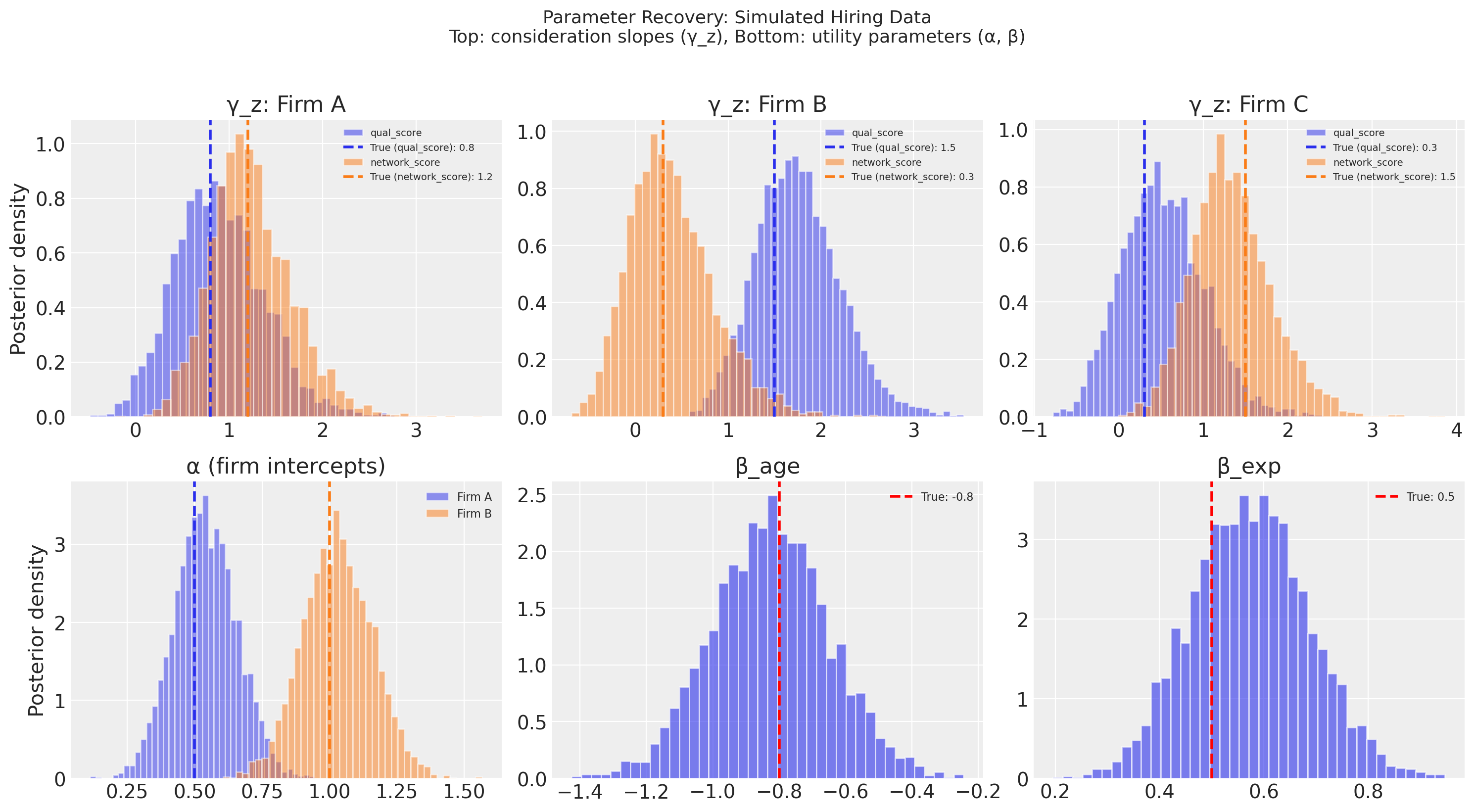
The model recovers both stages. The dashed lines (true values) fall within the posterior mass for all parameters. The consideration slopes are cleanly separated from the utility weights because the exclusion restriction holds by construction: qualification and network scores affect screening, while age and experience affect evaluation.

Now consider the counterfactual that motivated the hiring example. What happens if we widen the consideration set by giving every candidate a strong network score (+1 SD)? We shift network_score to 1.0 for all candidates, leaving qualification screening intact. This simulates a policy that connects every candidate equally to professional networks — candidates who previously had weak networks gain access, and the model shows which firms benefit most.

# ---- Counterfactual: give every candidate a strong network score (+1 SD) ----
# Baseline: posterior predictive with original instruments
model_sim.sample_posterior_predictive(random_seed=SEED)

# Counterfactual: shift network_score to +1 SD for all candidates
Z_tilde_strong_network = Z_tilde_3d_sim.copy()
Z_tilde_strong_network[:, :, 1] = 1.0  # everyone at +1 SD on network

idata_strong_network = model_sim.apply_intervention(
    new_choice_df=df_sim,
    new_consideration_instruments={
        "Z_tilde": Z_tilde_strong_network,
        "z_instrument_names": ["qual_score", "network_score"],
    },
)

# Compare market shares
p_base = model_sim.idata.posterior_predictive["p"].mean(dim=["chain", "draw"]).values
p_cf = idata_strong_network.posterior_predictive["p"].mean(dim=["chain", "draw"]).values

share_base = p_base.mean(axis=0)
share_cf = p_cf.mean(axis=0)

sim_share_df = pd.DataFrame(
    {
        "Firm": firm_names,
        "Baseline Share": share_base,
        "Strong-Network Share": share_cf,
        "Change": share_cf - share_base,
        "% Change": 100 * (share_cf - share_base) / share_base,
    }
).round(4)

print("Counterfactual: everyone at +1 SD network score")
sim_share_df

Sampling: [likelihood]

Sampling: [likelihood]

Counterfactual: everyone at +1 SD network score

	Firm	Baseline Share	Strong-Network Share	Change	% Change
0	Firm A	0.3148	0.3714	0.0566	17.9808
1	Firm B	0.4850	0.3896	-0.0954	-19.6712
2	Firm C	0.2002	0.2390	0.0388	19.3780

The shift in market shares reflects the structure we built in. Firm C (γ_network = 1.5) gains the most in relative terms (+19%) — it screens most heavily on network, so boosting everyone’s network score raises Firm C’s consideration probability most. Firm A (γ_network = 1.2) gains substantially as well (+18%).

Firm B (γ_network = 0.3), which barely screens on network, gains almost nothing from the boost. Because shares must sum to one, it absorbs the full displacement cost: it loses roughly 20% of its baseline share. The mechanism is market-share arithmetic — when two firms with high network sensitivity both expand, a third firm that is insensitive to the instrument bears the brunt of the reallocation, even though its own consideration probability is largely unchanged.

The counterfactual is credible here because the exclusion restriction holds by construction: network connections affect screening, not productivity conditional on evaluation. The model correctly decomposes the two channels — and the direction and magnitude of the effects follow directly from the recovered γ values.

This is the benchmark. When we turn to the Swiss Metro data below, the instruments are messier (GA proxies for lifestyle, not just awareness) and the exclusion restriction is debatable. The parameter recovery exercise establishes that the model works when its assumptions hold. The empirical application then asks what happens when they are strained.

---

Loading and Exploring the Swiss Metro Data

The Swiss Metro dataset is a stated-preference survey. Respondents choose between Train, SwissMetro (a hypothetical high-speed rail), and Car across 9 choice scenarios with varying travel times, costs, headways, and seat configurations.

data_path = data_dir / "swissmetro.dat"
raw = pd.read_csv(data_path, sep="\t")

# Standard filter: stated preference observations with valid choices
df = raw[(raw["SP"] == 1) & (raw["CHOICE"] != 0)].copy()
print(f"Observations: {len(df):,}")
print(f"Unique individuals: {df['ID'].nunique():,}")
print(f"Observations per individual: {len(df) // df['ID'].nunique()}")
print("\nChoice distribution:")
choice_map = {1: "Train", 2: "SwissMetro", 3: "Car"}
print(df["CHOICE"].map(choice_map).value_counts().sort_index())
car_unavail = (df["CAR_AV"] == 0).sum()
car_pct = 100 * (df["CAR_AV"] == 0).mean()
print(f"\nCar unavailable in {car_unavail:,} / {len(df):,} obs ({car_pct:.1f}%)")

Observations: 10,719
Unique individuals: 1,191
Observations per individual: 9

Choice distribution:
CHOICE
Car           3080
SwissMetro    6216
Train         1423
Name: count, dtype: int64

Car unavailable in 1,683 / 10,719 obs (15.7%)

Data Preprocessing

We prepare the data in wide format: string choice labels, scaled travel times and costs for numerical stability, and a subsample for tractable MCMC.

# Create string choice labels
df["choice"] = df["CHOICE"].map(choice_map)

# Scale covariates for numerical stability
df["train_tt"] = df["TRAIN_TT"] / 100  # travel time in units of 100 min
df["train_co"] = df["TRAIN_CO"] / 100  # cost in CHF
df["sm_tt"] = df["SM_TT"] / 100
df["sm_co"] = df["SM_CO"] / 100
df["car_tt"] = df["CAR_TT"] / 100
df["car_co"] = df["CAR_CO"] / 100

# Subsample for tractable notebook demonstration
# Take a random subset of individuals (preserving panel structure)
sampled_ids = rng.choice(df["ID"].unique(), size=250, replace=False)
df_sub = df[df["ID"].isin(sampled_ids)].copy().reset_index(drop=True)

print(
    f"Subsampled: {len(df_sub):,} observations from {df_sub['ID'].nunique()} individuals"
)
print("\nChoice distribution (subsample):")
print(df_sub["choice"].value_counts().sort_index())
df_sub[
    [
        "ID",
        "choice",
        "train_tt",
        "train_co",
        "sm_tt",
        "sm_co",
        "car_tt",
        "car_co",
        "TRAIN_HE",
        "SM_HE",
        "CAR_AV",
        "GA",
    ]
].head(6)

Subsampled: 2,250 observations from 250 individuals

Choice distribution (subsample):
choice
Car            634
SwissMetro    1314
Train          302
Name: count, dtype: int64

	ID	choice	train_tt	train_co	sm_tt	sm_co	car_tt	car_co	TRAIN_HE	SM_HE	CAR_AV	GA
0	8	SwissMetro	1.09	0.26	0.56	0.34	1.3	0.30	120	20	1	0
1	8	SwissMetro	1.00	0.26	0.53	0.32	1.3	0.39	30	10	1	0
2	8	SwissMetro	1.26	0.26	0.60	0.40	1.3	0.24	60	30	1	0
3	8	Car	1.00	0.22	0.56	0.35	0.8	0.24	30	20	1	0
4	8	SwissMetro	1.26	0.20	0.56	0.24	1.0	0.39	60	20	1	0
5	8	Car	1.09	0.20	0.53	0.32	1.0	0.24	120	10	1	0

Constructing Consideration Instruments

The consideration instruments must satisfy the exclusion restriction: they should affect whether a mode enters the consideration set, not utility conditional on consideration. Without this separation, the model cannot distinguish “didn’t notice” from “noticed but disliked.”

We use four person-level characteristics. Each captures a reason why someone’s streetlamp might point in a particular direction.

GA (General Abonnement) is an annual rail pass. Holders are habituated to rail. The pass doesn’t change how fast or cheap a trip is; it changes whether rail is on the radar. A subscription buys you into a consideration set. Business indicates a business trip. Business travellers may default to employer-reimbursed modes or familiar routines, narrowing consideration before any evaluation of time or cost. High income flags household income above the median. Higher income may expand the consideration set: more modes feel affordable enough to think about. Older flags respondents above the median age, who may have entrenched habits that restrict active consideration.

The key feature is that gamma_z varies by mode. A GA pass may strongly increase Train consideration while having no effect on Car. The model learns these mode-specific sensitivities from the data.

# ---- Person-level consideration instruments ----
ga = df_sub["GA"].values.astype(float)
business = (df_sub["PURPOSE"] == 1).values.astype(float)
high_inc = (df_sub["INCOME"] > 2).values.astype(float)
older = (df_sub["AGE"] > 3).values.astype(float)

# Composite Z: same instruments for each mode, but gamma varies by mode
Z_person = np.column_stack([ga, business, high_inc, older])  # (N, 4)
Z_means = Z_person.mean(axis=0)
Z_tilde_person = Z_person - Z_means  # mean-centred

# Stack to (N, J, K_z) — same person-level Z for all modes
# gamma_z[j, k] will learn mode-specific sensitivities
n_alts = 3
Z_tilde = np.stack([Z_tilde_person] * n_alts, axis=1)  # (N, 3, 4)

z_names = ["GA", "Business", "High_income", "Older"]

print(f"Z_tilde shape: {Z_tilde.shape}  (N, J, K_z)")
print("\nInstrument means (pre-centring):")
for name, m in zip(z_names, Z_means, strict=True):
    print(f"  {name:12s}: {m:.3f}")
print(f"\nZ_tilde column means (should be ~0): {Z_tilde_person.mean(axis=0).round(6)}")

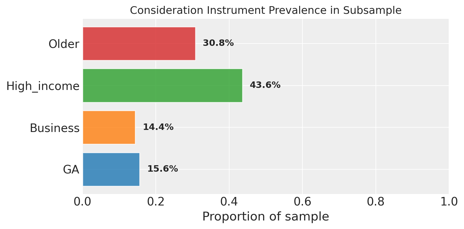
Z_tilde shape: (2250, 3, 4)  (N, J, K_z)

Instrument means (pre-centring):
  GA          : 0.156
  Business    : 0.144
  High_income : 0.436
  Older       : 0.308

Z_tilde column means (should be ~0): [-0. -0. -0. -0.]

Show code cell source

Hide code cell source

# Instrument prevalence (pre-centring) — proportion of sample with each trait
instrument_rates = Z_means
fig, ax = plt.subplots(figsize=(8, 4))
colors = ["#1f77b4", "#ff7f0e", "#2ca02c", "#d62728"]
bars = ax.barh(z_names, instrument_rates, color=colors, alpha=0.8, edgecolor="white")
ax.set_xlim(0, 1)
ax.set_xlabel("Proportion of sample")
ax.set_title("Consideration Instrument Prevalence in Subsample", fontsize=13)
for bar, rate in zip(bars, instrument_rates, strict=True):
    ax.text(
        rate + 0.02,
        bar.get_y() + bar.get_height() / 2,
        f"{rate:.1%}",
        va="center",
        fontsize=11,
        fontweight="bold",
    )
plt.tight_layout()

/var/folders/__/ng_3_9pn1f11ftyml_qr69vh0000gn/T/ipykernel_79640/1470404791.py:18: UserWarning: The figure layout has changed to tight
  plt.tight_layout()

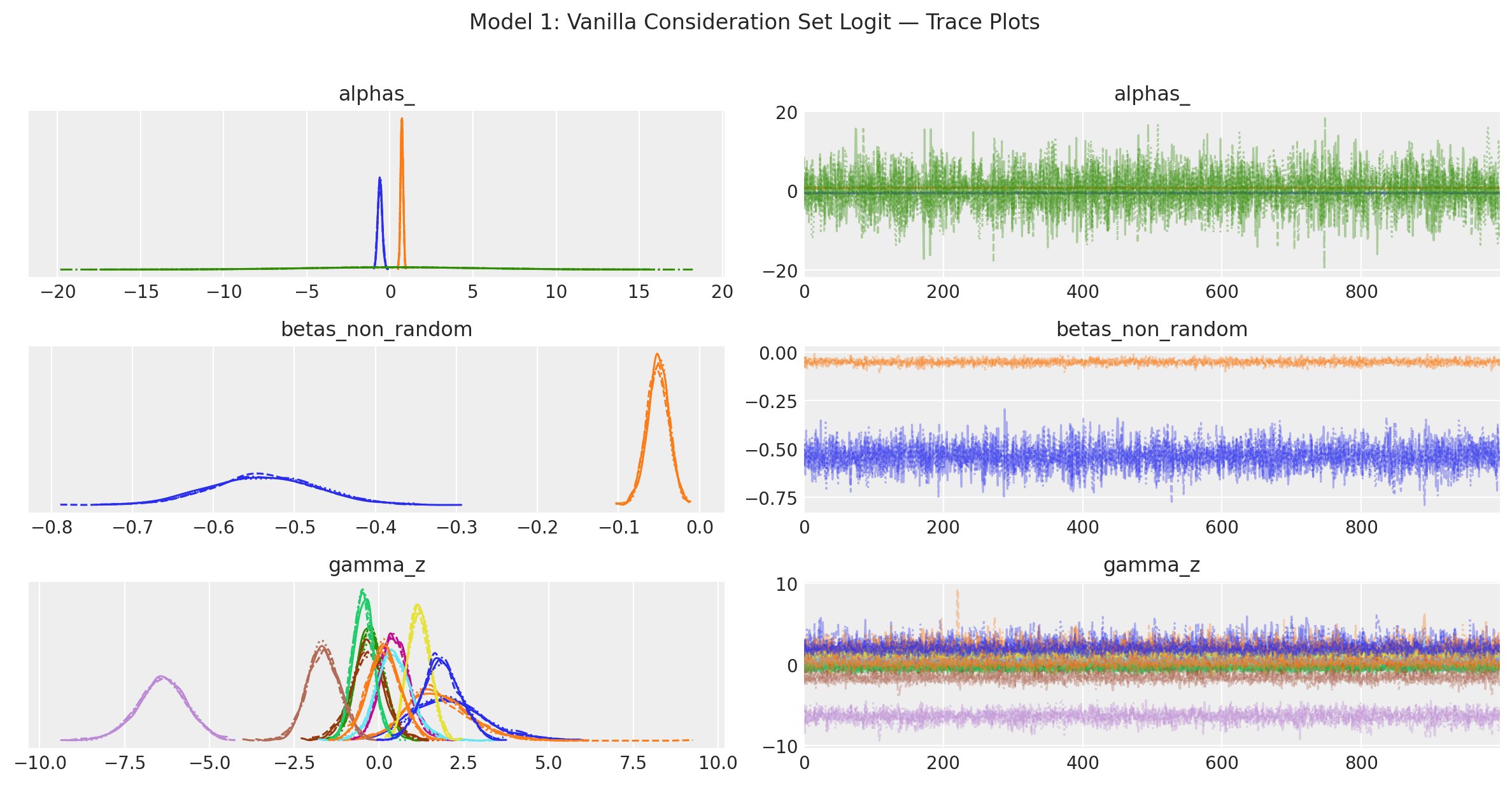
Model 1: Vanilla Consideration Set Logit (No Random Effects)

Our first model uses fixed coefficients for travel time and cost. This is the simplest consideration set model: a consideration stage on top of a standard conditional logit. Travel time and cost are alternative-specific covariates, varying across modes within each choice scenario.

# Utility equations: alternative ~ alt_specific_covariates
# No fixed (individual-level) covariates, no random covariates
utility_equations = [
    "Train ~ train_tt + train_co",
    "SwissMetro ~ sm_tt + sm_co",
    "Car ~ car_tt + car_co",
]

model_vanilla = ConsiderationSetMixedLogit(
    choice_df=df_sub,
    utility_equations=utility_equations,
    depvar="choice",
    covariates=["tt", "co"],
    consideration_instruments={
        "Z_tilde": Z_tilde,
        "z_instrument_names": z_names,
    },
    consideration_intercept=False,  # default: utility intercepts absorb baseline
    random_consideration=False,
    group_id="ID",
    sampler_config={
        "target_accept": 0.95,
        "tune": 1000,
        "draws": 1000,
        "chains": 4,
        "cores": 4,
        "nuts_sampler": "pymc",
    },
)

model_vanilla.build_model()
print("Model 1 (vanilla consideration) free RVs:")
print([v.name for v in model_vanilla.model.free_RVs])
print("\nDeterministics:")
print([v.name for v in model_vanilla.model.deterministics])

Model 1 (vanilla consideration) free RVs:
['alphas_', 'betas_non_random', 'gamma_z']

Deterministics:
['alphas', 'betas_individuals', 'U', 'pi', 'p']

pm.model_to_graphviz(model_vanilla.model)

idata_vanilla = model_vanilla.fit(
    idata_kwargs={"log_likelihood": True},
    random_seed=SEED,
    fit_kwargs={
        "target_accept": 0.95,
        "tune": 1000,
        "draws": 1000,
        "chains": 4,
        "cores": 4,
    },
)

Initializing NUTS using jitter+adapt_diag...
Multiprocess sampling (4 chains in 4 jobs)
NUTS: [alphas_, betas_non_random, gamma_z]
/Users/nathanielforde/mambaforge/envs/pymc-marketing-dev/lib/python3.12/multiprocessing/popen_fork.py:66: RuntimeWarning: os.fork() was called. os.fork() is incompatible with multithreaded code, and JAX is multithreaded, so this will likely lead to a deadlock.
  self.pid = os.fork()

/Users/nathanielforde/mambaforge/envs/pymc-marketing-dev/lib/python3.12/multiprocessing/popen_fork.py:66: RuntimeWarning: os.fork() was called. os.fork() is incompatible with multithreaded code, and JAX is multithreaded, so this will likely lead to a deadlock.
  self.pid = os.fork()

Sampling 4 chains for 1_000 tune and 1_000 draw iterations (4_000 + 4_000 draws total) took 53 seconds.

var_names_vanilla = ["alphas_", "betas_non_random", "gamma_z"]
az.summary(idata_vanilla, var_names=var_names_vanilla, round_to=3)

	mean	sd	hdi_3%	hdi_97%	mcse_mean	mcse_sd	ess_bulk	ess_tail	r_hat
alphas_[Train]	-0.594	0.129	-0.829	-0.346	0.003	0.002	2276.126	2381.439	1.001
alphas_[SwissMetro]	0.720	0.077	0.589	0.876	0.001	0.001	2687.265	2484.053	1.000
alphas_[Car]	0.095	5.036	-9.317	9.542	0.073	0.089	4811.485	2484.541	1.000
betas_non_random[tt]	-0.537	0.066	-0.655	-0.409	0.001	0.001	4771.644	2851.436	1.003
betas_non_random[co]	-0.051	0.013	-0.076	-0.026	0.000	0.000	2610.659	2531.973	1.002
gamma_z[Train, GA]	2.043	1.086	0.161	4.288	0.023	0.020	2121.835	1838.897	1.001
gamma_z[Train, Business]	1.714	0.961	0.109	3.732	0.020	0.023	2354.629	2206.043	1.001
gamma_z[Train, High_income]	-0.260	0.399	-0.985	0.502	0.008	0.006	2614.373	2507.947	1.000
gamma_z[Train, Older]	0.484	0.428	-0.336	1.278	0.008	0.007	2986.114	2456.809	1.001
gamma_z[SwissMetro, GA]	-0.321	0.509	-1.288	0.640	0.011	0.010	2258.773	2053.726	1.001
gamma_z[SwissMetro, Business]	0.439	0.535	-0.543	1.478	0.011	0.013	2455.602	2144.509	1.001
gamma_z[SwissMetro, High_income]	1.179	0.331	0.589	1.819	0.007	0.005	2570.198	2412.804	1.000
gamma_z[SwissMetro, Older]	-0.463	0.307	-1.044	0.117	0.006	0.005	2707.653	2457.214	1.001
gamma_z[Car, GA]	-6.403	0.720	-7.743	-5.031	0.014	0.015	2560.925	1843.876	1.003
gamma_z[Car, Business]	-1.653	0.480	-2.508	-0.736	0.010	0.009	2556.422	2335.578	1.000
gamma_z[Car, High_income]	1.850	0.551	0.850	2.913	0.010	0.009	2840.736	2425.817	1.000
gamma_z[Car, Older]	0.159	0.482	-0.743	1.082	0.009	0.007	2746.006	2859.048	1.001

Show code cell source

Hide code cell source

axes = az.plot_trace(idata_vanilla, var_names=var_names_vanilla, compact=True)
plt.suptitle("Model 1: Vanilla Consideration Set Logit — Trace Plots", y=1.02)
plt.tight_layout()

/var/folders/__/ng_3_9pn1f11ftyml_qr69vh0000gn/T/ipykernel_79640/2572815254.py:3: UserWarning: The figure layout has changed to tight
  plt.tight_layout()

Interpreting the Consideration Stage

The gamma_z parameters answer the question: what determines where the streetlamp shines? We have 4 instruments and 3 modes, giving 12 screening slopes. A positive gamma_z means the instrument increases consideration of that mode. Where these slopes are large relative to utility parameters, consideration is the primary driver of choice. That is the audit signal.

Show code cell source

Hide code cell source

# ---- Consideration parameters: gamma_z by mode (4 instruments each) ----
# gamma_z has dims (alts, z_instruments) → each mode gets 4 slopes
alt_names = list(idata_vanilla.posterior.coords["alts"].values)

fig, axes = plt.subplots(1, 3, figsize=(16, 4.5))
colors = ["#1f77b4", "#ff7f0e", "#2ca02c", "#d62728"]

for j, (ax, mode) in enumerate(zip(axes, alt_names, strict=True)):
    gamma_post = idata_vanilla.posterior["gamma_z"].sel(alts=mode)
    for k, z_name in enumerate(z_names):
        samples = gamma_post.sel(z_instruments=z_name).values.flatten()
        ax.hist(
            samples,
            bins=40,
            alpha=0.55,
            label=z_name,
            density=True,
            color=colors[k],
            edgecolor="white",
        )
    ax.axvline(0, color="black", linestyle="--", alpha=0.5, linewidth=1)
    ax.set_title(f"γ_z: {mode}", fontsize=12)
    ax.set_xlabel("Consideration slope")
    if j == 0:
        ax.set_ylabel("Posterior density")
    ax.legend(fontsize=8)

plt.suptitle(
    "Consideration Screening Parameters γ_z by Mode\n"
    "Positive = instrument increases consideration probability",
    y=1.05,
    fontsize=13,
)
plt.tight_layout()

/var/folders/__/ng_3_9pn1f11ftyml_qr69vh0000gn/T/ipykernel_79640/2213030523.py:34: UserWarning: The figure layout has changed to tight
  plt.tight_layout()

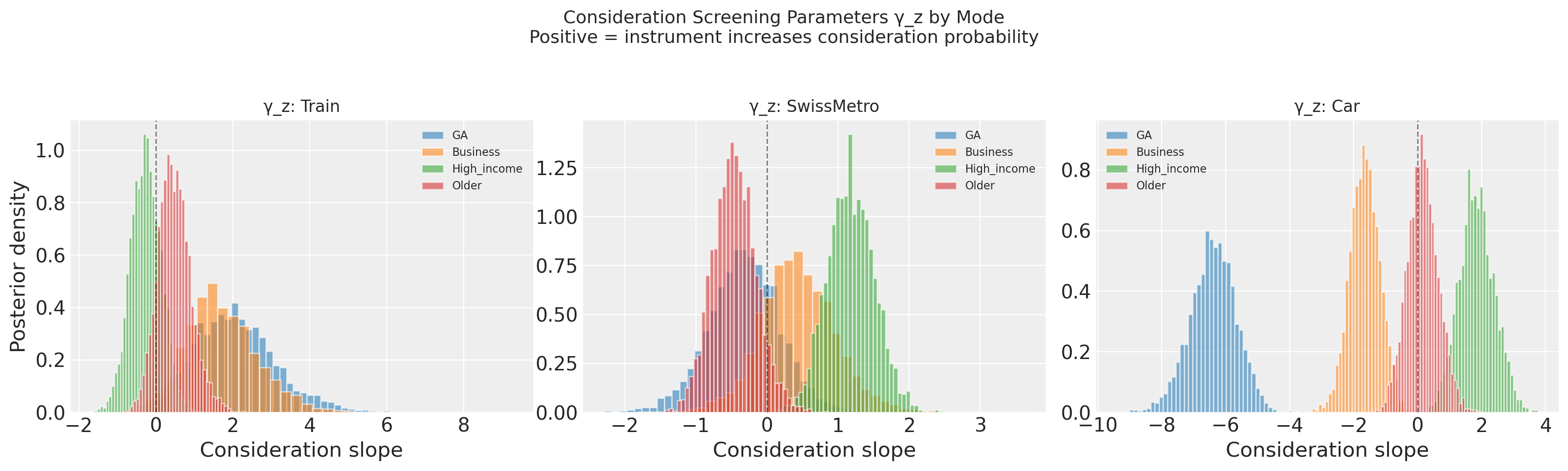
GA dominates. It strongly increases consideration of Train and SwissMetro (rail pass holders have rail on their radar) and strongly decreases Car consideration (GA holders are rail-embedded). Business and Older show more diffuse effects, suggesting weaker screening. High_income effects are moderate and mode-dependent.

Note the scale. GA slopes run ±5 to ±10; the utility-stage coefficients below are much smaller. For this population, who considers what matters at least as much as how they evaluate it.

Show code cell source

Hide code cell source

# ---- Utility-stage parameters ----
az.plot_posterior(
    idata_vanilla,
    var_names=["alphas_", "betas_non_random"],
    figsize=(12, 6),
)
plt.suptitle(
    "Utility Stage: Mode Constants (α) and Covariate Sensitivities (β)\n"
    "Expected: negative β_tt (prefer faster), negative β_co (prefer cheaper)",
    y=1.05,
)
plt.tight_layout()

/var/folders/__/ng_3_9pn1f11ftyml_qr69vh0000gn/T/ipykernel_79640/2366119182.py:12: UserWarning: The figure layout has changed to tight
  plt.tight_layout()

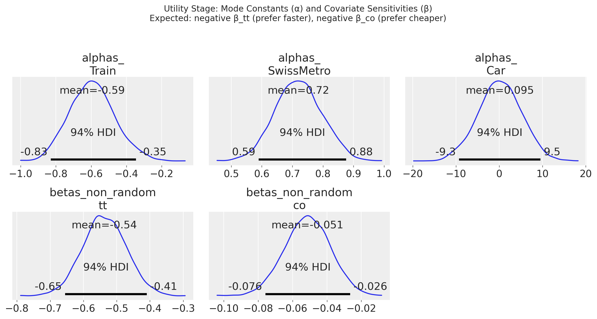
The utility-stage parameters behave as expected. Both travel time and cost coefficients are negative: people prefer faster and cheaper options. The mode constants capture baseline preference after accounting for time and cost. These are the “rational evaluation” parameters, operating conditional on consideration.

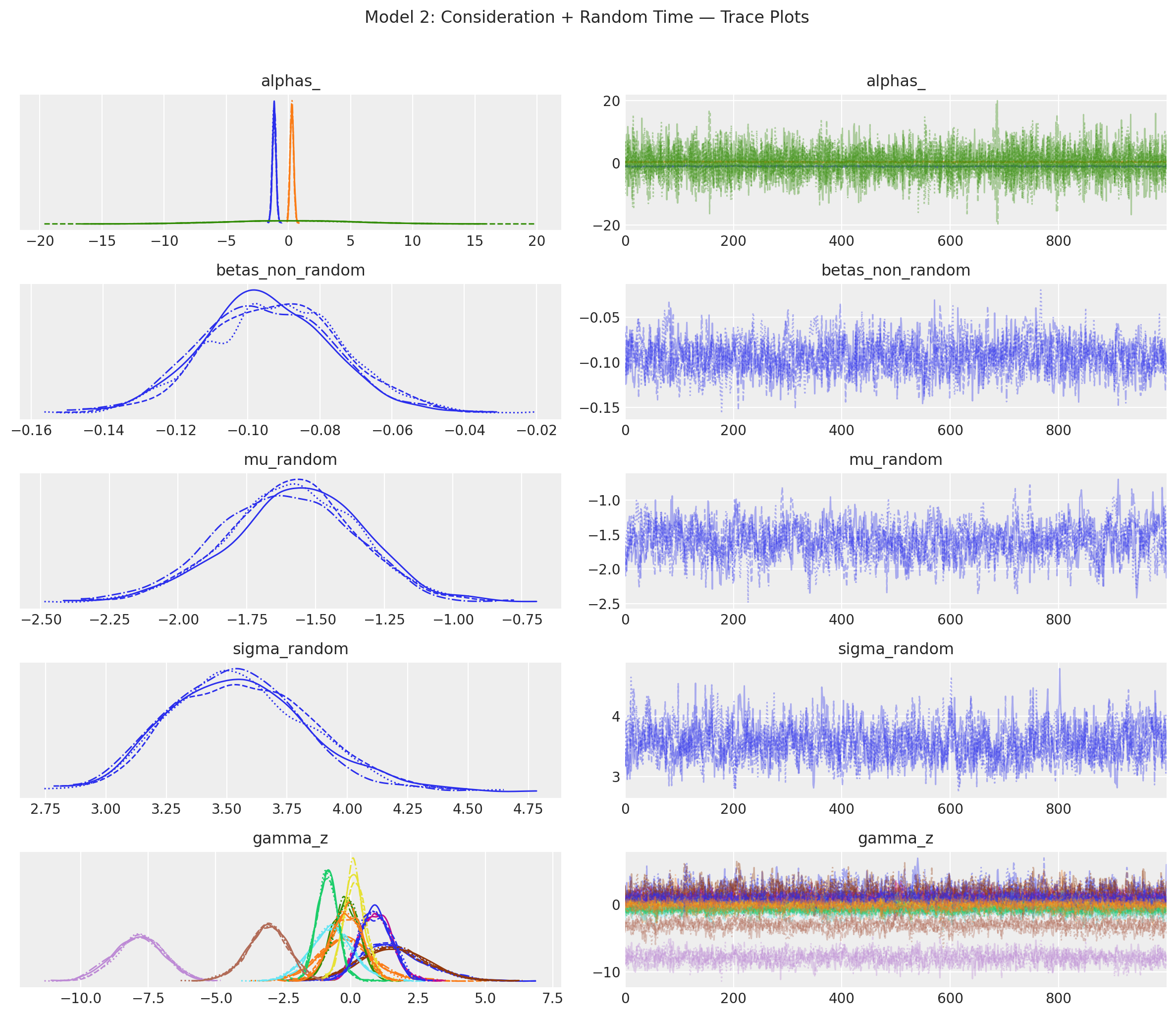
Model 2: Consideration Set Logit with Random Effects on Travel Time

We now allow taste heterogeneity in time sensitivity. Some individuals are time-sensitive business travellers; others accept longer journeys. The random coefficient \(\beta^{tt}_n \sim \mathcal{N}(\mu_{tt}, \sigma_{tt}^2)\) is integrated out in the marginal likelihood:

\[P(y_n = j) = \int \frac{\pi_{nj} \cdot \exp(V_{nj}(\beta^{tt}_n))}{\sum_k \pi_{nk} \cdot \exp(V_{nk}(\beta^{tt}_n))} \, \phi(\beta^{tt}_n \mid \mu_{tt}, \sigma_{tt}) \, d\beta^{tt}_n\]

MCMC draws individual-level \(\beta^{tt}_n\) values, computing this integral through sampling.

# Travel time is now a random coefficient (third part of formula after ||)
# Cost remains fixed
utility_equations_random = [
    "Train ~ train_tt + train_co | | train_tt",
    "SwissMetro ~ sm_tt + sm_co | | sm_tt",
    "Car ~ car_tt + car_co | | car_tt",
]

model_random = ConsiderationSetMixedLogit(
    choice_df=df_sub,
    utility_equations=utility_equations_random,
    depvar="choice",
    covariates=["tt", "co"],
    consideration_instruments={
        "Z_tilde": Z_tilde,
        "z_instrument_names": z_names,
    },
    consideration_intercept=False,
    random_consideration=False,
    group_id="ID",
    non_centered=True,  # better mixing for hierarchical models
)

model_random.build_model()
print("Model 2 (random time) free RVs:")
print([v.name for v in model_random.model.free_RVs])

Model 2 (random time) free RVs:
['alphas_', 'betas_non_random', 'mu_random', 'sigma_random', 'z_random_group', 'gamma_z']

pm.model_to_graphviz(model_random.model)

idata_random = model_random.fit(
    target_accept=0.95,
    draws=1000,
    tune=1000,
    chains=4,
    idata_kwargs={"log_likelihood": True},
    nuts_sampler="nutpie",
    random_seed=SEED,
)

# Generate posterior predictive (needed for baseline market shares later)
model_random.sample_posterior_predictive()

/Users/nathanielforde/mambaforge/envs/pymc-marketing-dev/lib/python3.12/site-packages/pymc/sampling/mcmc.py:361: UserWarning: `idata_kwargs` are currently ignored by the nutpie sampler
  warnings.warn(

Sampler Progress

Total Chains: 4

Active Chains: 0

Finished Chains: 4

Sampling for 41 seconds

Estimated Time to Completion: now

Progress	Draws	Divergences	Step Size	Gradients/Draw
	2000	0	0.16	31
	2000	0	0.13	31
	2000	0	0.16	31
	2000	0	0.16	31

Sampling: [likelihood]

arviz.InferenceData

• posterior_predictive

  <xarray.Dataset> Size: 288MB
  Dimensions:     (chain: 4, draw: 1000, obs: 2250, alts: 3)
  Coordinates:
    * chain       (chain) int64 32B 0 1 2 3
    * draw        (draw) int64 8kB 0 1 2 3 4 5 6 7 ... 993 994 995 996 997 998 999
    * obs         (obs) int64 18kB 0 1 2 3 4 5 6 ... 2244 2245 2246 2247 2248 2249
    * alts        (alts) <U10 120B 'Train' 'SwissMetro' 'Car'
  Data variables:
      likelihood  (chain, draw, obs) int64 72MB 1 1 1 2 1 1 2 2 ... 2 1 1 1 1 1 1
      p           (chain, draw, obs, alts) float64 216MB 0.1501 0.739 ... 0.1638
  Attributes:
      created_at:                 2026-04-19T22:13:36.315913+00:00
      arviz_version:              0.23.0
      inference_library:          pymc
      inference_library_version:  5.28.2

  xarray.Dataset

  • Dimensions:
    • chain: 4
    • draw: 1000
    • obs: 2250
    • alts: 3
  • Coordinates: (4)
    • chain
      (chain)
      int64
      0 1 2 3

      array([0, 1, 2, 3])

    • draw
      (draw)
      int64
      0 1 2 3 4 5 ... 995 996 997 998 999

      array([  0,   1,   2, ..., 997, 998, 999], shape=(1000,))

    • obs
      (obs)
      int64
      0 1 2 3 4 ... 2246 2247 2248 2249

      array([   0,    1,    2, ..., 2247, 2248, 2249], shape=(2250,))

    • alts
      (alts)
      <U10
      'Train' 'SwissMetro' 'Car'

      array(['Train', 'SwissMetro', 'Car'], dtype='<U10')

  • Data variables: (2)
    • likelihood
      (chain, draw, obs)
      int64
      1 1 1 2 1 1 2 2 ... 1 2 1 1 1 1 1 1

      array([[[1, 1, 1, ..., 1, 1, 1],
              [1, 1, 1, ..., 1, 1, 1],
              [1, 1, 1, ..., 1, 1, 1],
              ...,
              [2, 1, 1, ..., 1, 1, 1],
              [0, 1, 1, ..., 1, 1, 1],
              [0, 1, 0, ..., 1, 1, 1]],
      
             [[1, 1, 2, ..., 1, 1, 1],
              [1, 1, 1, ..., 2, 1, 1],
              [1, 1, 1, ..., 1, 1, 1],
              ...,
              [1, 1, 1, ..., 1, 1, 1],
              [1, 0, 1, ..., 1, 1, 2],
              [1, 1, 1, ..., 1, 1, 1]],
      
             [[2, 1, 1, ..., 1, 1, 1],
              [1, 1, 1, ..., 1, 2, 1],
              [1, 1, 1, ..., 2, 2, 1],
              ...,
              [1, 0, 2, ..., 2, 1, 1],
              [1, 1, 1, ..., 1, 1, 1],
              [1, 1, 2, ..., 0, 1, 1]],
      
             [[1, 1, 1, ..., 1, 1, 2],
              [1, 2, 1, ..., 1, 1, 2],
              [1, 1, 1, ..., 2, 1, 1],
              ...,
              [1, 0, 1, ..., 1, 1, 1],
              [1, 1, 1, ..., 1, 1, 1],
              [1, 1, 1, ..., 1, 1, 1]]], shape=(4, 1000, 2250))

    • p
      (chain, draw, obs, alts)
      float64
      0.1501 0.739 ... 0.8154 0.1638

      array([[[[1.50058558e-01, 7.38963429e-01, 1.10978012e-01],
               [1.83283127e-01, 7.21090956e-01, 9.56259172e-02],
               [9.60655862e-02, 7.68130222e-01, 1.35804191e-01],
               ...,
               [9.93947762e-03, 9.26089214e-01, 6.39713083e-02],
               [8.62711378e-03, 9.37837144e-01, 5.35357419e-02],
               [8.43867863e-03, 9.15495396e-01, 7.60659253e-02]],
      
              [[8.95465699e-02, 8.66754620e-01, 4.36988103e-02],
               [1.06750829e-01, 8.54642343e-01, 3.86068280e-02],
               [6.08977399e-02, 8.87474677e-01, 5.16275833e-02],
               ...,
               [1.99734455e-02, 8.01826734e-01, 1.78199821e-01],
               [1.85851894e-02, 8.22855719e-01, 1.58559092e-01],
               [1.78362425e-02, 7.87735865e-01, 1.94427892e-01]],
      
              [[1.17936087e-01, 8.21948742e-01, 6.01151708e-02],
               [1.39037104e-01, 8.07811668e-01, 5.31512284e-02],
               [8.20887779e-02, 8.46829890e-01, 7.10813323e-02],
               ...,
      ...
               [1.46866669e-02, 8.62517545e-01, 1.22795788e-01],
               [1.33523513e-02, 8.78811073e-01, 1.07836576e-01],
               [1.29260981e-02, 8.49119867e-01, 1.37954035e-01]],
      
              [[1.53899134e-02, 9.80597316e-01, 4.01277030e-03],
               [2.21772099e-02, 9.74546657e-01, 3.27613334e-03],
               [6.94170463e-03, 9.87816962e-01, 5.24133354e-03],
               ...,
               [2.80336252e-02, 7.99048613e-01, 1.72917762e-01],
               [2.60929753e-02, 8.18117541e-01, 1.55789484e-01],
               [2.50969004e-02, 7.85464044e-01, 1.89439055e-01]],
      
              [[1.35286517e-02, 9.74341222e-01, 1.21301265e-02],
               [2.03179100e-02, 9.69972119e-01, 9.70997116e-03],
               [5.58208152e-03, 9.78176256e-01, 1.62416625e-02],
               ...,
               [2.32257205e-02, 8.27628821e-01, 1.49145458e-01],
               [2.15166645e-02, 8.45378571e-01, 1.33104765e-01],
               [2.07963163e-02, 8.15382652e-01, 1.63821032e-01]]]],
            shape=(4, 1000, 2250, 3))

  • Attributes: (4)

    created_at :

    2026-04-19T22:13:36.315913+00:00

    arviz_version :

    0.23.0

    inference_library :

    pymc

    inference_library_version :

    5.28.2

  
  
• observed_data

  <xarray.Dataset> Size: 36kB
  Dimensions:     (obs: 2250)
  Coordinates:
    * obs         (obs) int64 18kB 0 1 2 3 4 5 6 ... 2244 2245 2246 2247 2248 2249
  Data variables:
      likelihood  (obs) int64 18kB 1 1 1 2 1 2 2 1 1 1 1 ... 2 2 1 1 1 1 1 1 1 1 0
  Attributes:
      created_at:                 2026-04-19T22:13:36.320879+00:00
      arviz_version:              0.23.0
      inference_library:          pymc
      inference_library_version:  5.28.2

  xarray.Dataset

  • Dimensions:
    • obs: 2250
  • Coordinates: (1)
    • obs
      (obs)
      int64
      0 1 2 3 4 ... 2246 2247 2248 2249

      array([   0,    1,    2, ..., 2247, 2248, 2249], shape=(2250,))

  • Data variables: (1)
    • likelihood
      (obs)
      int64
      1 1 1 2 1 2 2 1 ... 1 1 1 1 1 1 1 0

      array([1, 1, 1, ..., 1, 1, 0], shape=(2250,))

  • Attributes: (4)

    created_at :

    2026-04-19T22:13:36.320879+00:00

    arviz_version :

    0.23.0

    inference_library :

    pymc

    inference_library_version :

    5.28.2

  
  
• constant_data

  <xarray.Dataset> Size: 360kB
  Dimensions:        (obs: 2250, alts: 3, covariates: 2, z_instruments: 4)
  Coordinates:
    * obs            (obs) int64 18kB 0 1 2 3 4 5 ... 2245 2246 2247 2248 2249
    * alts           (alts) <U10 120B 'Train' 'SwissMetro' 'Car'
    * covariates     (covariates) <U2 16B 'tt' 'co'
    * z_instruments  (z_instruments) <U11 176B 'GA' 'Business' ... 'Older'
  Data variables:
      X              (obs, alts, covariates) float64 108kB 1.09 0.26 ... 0.9 0.84
      Z              (obs, alts, z_instruments) float64 216kB -0.156 ... -0.308
      y              (obs) int32 9kB 1 1 1 2 1 2 2 1 1 1 1 ... 2 1 1 1 1 1 1 1 1 0
      grp_idx        (obs) int32 9kB 0 0 0 0 0 0 0 ... 249 249 249 249 249 249 249
  Attributes:
      created_at:                 2026-04-19T22:13:36.323592+00:00
      arviz_version:              0.23.0
      inference_library:          pymc
      inference_library_version:  5.28.2

  xarray.Dataset

  • Dimensions:
    • obs: 2250
    • alts: 3
    • covariates: 2
    • z_instruments: 4
  • Coordinates: (4)
    • obs
      (obs)
      int64
      0 1 2 3 4 ... 2246 2247 2248 2249

      array([   0,    1,    2, ..., 2247, 2248, 2249], shape=(2250,))

    • alts
      (alts)
      <U10
      'Train' 'SwissMetro' 'Car'

      array(['Train', 'SwissMetro', 'Car'], dtype='<U10')

    • covariates
      (covariates)
      <U2
      'tt' 'co'

      array(['tt', 'co'], dtype='<U2')

    • z_instruments
      (z_instruments)
      <U11
      'GA' 'Business' ... 'Older'

      array(['GA', 'Business', 'High_income', 'Older'], dtype='<U11')

  • Data variables: (4)
    • X
      (obs, alts, covariates)
      float64
      1.09 0.26 0.56 ... 0.31 0.9 0.84

      array([[[1.09, 0.26],
              [0.56, 0.34],
              [1.3 , 0.3 ]],
      
             [[1.  , 0.26],
              [0.53, 0.32],
              [1.3 , 0.39]],
      
             [[1.26, 0.26],
              [0.6 , 0.4 ],
              [1.3 , 0.24]],
      
             ...,
      
             [[0.85, 0.23],
              [0.37, 0.25],
              [0.9 , 0.52]],
      
             [[0.85, 0.19],
              [0.34, 0.25],
              [0.9 , 0.84]],
      
             [[0.92, 0.23],
              [0.41, 0.31],
              [0.9 , 0.84]]], shape=(2250, 3, 2))

    • Z
      (obs, alts, z_instruments)
      float64
      -0.156 0.856 0.564 ... 0.564 -0.308

      array([[[-0.156,  0.856,  0.564,  0.692],
              [-0.156,  0.856,  0.564,  0.692],
              [-0.156,  0.856,  0.564,  0.692]],
      
             [[-0.156,  0.856,  0.564,  0.692],
              [-0.156,  0.856,  0.564,  0.692],
              [-0.156,  0.856,  0.564,  0.692]],
      
             [[-0.156,  0.856,  0.564,  0.692],
              [-0.156,  0.856,  0.564,  0.692],
              [-0.156,  0.856,  0.564,  0.692]],
      
             ...,
      
             [[-0.156, -0.144,  0.564, -0.308],
              [-0.156, -0.144,  0.564, -0.308],
              [-0.156, -0.144,  0.564, -0.308]],
      
             [[-0.156, -0.144,  0.564, -0.308],
              [-0.156, -0.144,  0.564, -0.308],
              [-0.156, -0.144,  0.564, -0.308]],
      
             [[-0.156, -0.144,  0.564, -0.308],
              [-0.156, -0.144,  0.564, -0.308],
              [-0.156, -0.144,  0.564, -0.308]]], shape=(2250, 3, 4))

    • y
      (obs)
      int32
      1 1 1 2 1 2 2 1 ... 1 1 1 1 1 1 1 0

      array([1, 1, 1, ..., 1, 1, 0], shape=(2250,), dtype=int32)

    • grp_idx
      (obs)
      int32
      0 0 0 0 0 0 ... 249 249 249 249 249

      array([  0,   0,   0, ..., 249, 249, 249], shape=(2250,), dtype=int32)

  • Attributes: (4)

    created_at :

    2026-04-19T22:13:36.323592+00:00

    arviz_version :

    0.23.0

    inference_library :

    pymc

    inference_library_version :

    5.28.2

  
  

var_names_random = [
    "alphas_",
    "betas_non_random",
    "mu_random",
    "sigma_random",
    "gamma_z",
]
az.summary(idata_random, var_names=var_names_random, round_to=3)

	mean	sd	hdi_3%	hdi_97%	mcse_mean	mcse_sd	ess_bulk	ess_tail	r_hat
alphas_[Train]	-1.140	0.150	-1.413	-0.843	0.004	0.003	1333.540	1758.391	1.003
alphas_[SwissMetro]	0.287	0.144	0.029	0.564	0.005	0.003	911.412	1447.955	1.005
alphas_[Car]	0.038	5.091	-9.725	9.280	0.052	0.095	9733.710	2667.255	1.003
betas_non_random[co]	-0.094	0.018	-0.128	-0.060	0.001	0.000	954.591	1267.820	1.005
mu_random[tt]	-1.590	0.243	-2.060	-1.155	0.011	0.005	515.654	1237.434	1.005
sigma_random[tt]	3.554	0.288	3.051	4.105	0.011	0.005	735.228	1804.411	1.003
gamma_z[Train, GA]	1.620	1.208	-0.660	3.880	0.038	0.022	1027.635	1621.070	1.002
gamma_z[Train, Business]	-0.162	1.033	-2.061	1.860	0.038	0.023	768.707	1335.895	1.004
gamma_z[Train, High_income]	-0.156	0.529	-1.196	0.799	0.013	0.008	1674.556	2486.573	1.001
gamma_z[Train, Older]	0.927	0.608	-0.155	2.066	0.015	0.012	1804.973	1896.168	1.002
gamma_z[SwissMetro, GA]	1.580	1.264	-0.760	3.924	0.043	0.024	848.640	1445.015	1.004
gamma_z[SwissMetro, Business]	-0.707	0.815	-2.276	0.828	0.030	0.018	733.430	1344.498	1.003
gamma_z[SwissMetro, High_income]	0.157	0.412	-0.592	0.957	0.011	0.007	1434.013	1827.321	1.004
gamma_z[SwissMetro, Older]	-0.854	0.403	-1.597	-0.131	0.012	0.012	1237.104	1613.259	1.000
gamma_z[Car, GA]	-7.844	0.922	-9.568	-6.117	0.026	0.014	1249.283	2095.862	1.002
gamma_z[Car, Business]	-3.079	0.764	-4.470	-1.558	0.028	0.015	735.592	1475.044	1.002
gamma_z[Car, High_income]	0.936	0.587	-0.077	2.094	0.014	0.009	1890.598	2180.579	1.002
gamma_z[Car, Older]	-0.153	0.601	-1.272	0.958	0.015	0.010	1535.970	2425.250	1.002

Show code cell source

Hide code cell source

axes = az.plot_trace(idata_random, var_names=var_names_random, compact=True)
plt.suptitle("Model 2: Consideration + Random Time — Trace Plots", y=1.02)
plt.tight_layout()

/var/folders/__/ng_3_9pn1f11ftyml_qr69vh0000gn/T/ipykernel_79640/195189237.py:3: UserWarning: The figure layout has changed to tight
  plt.tight_layout()

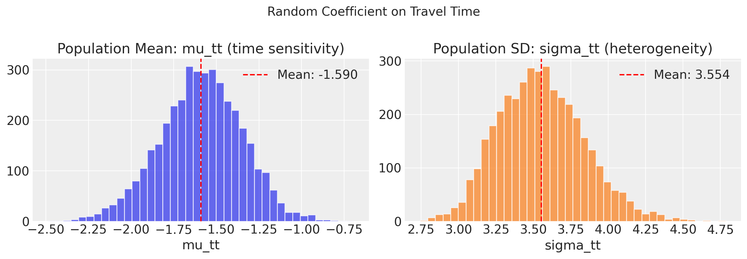
Individual-Level Heterogeneity in Time Sensitivity

The random coefficient on travel time captures taste heterogeneity. Below we plot the population distribution of individual-level time coefficients.

Show code cell source

Hide code cell source

# Plot the population distribution of random time coefficient
fig, axes = plt.subplots(1, 2, figsize=(12, 4))

# Population-level parameters
mu_tt = idata_random.posterior["mu_random"].sel(random_covariates="tt").values.flatten()
sigma_tt = (
    idata_random.posterior["sigma_random"].sel(random_covariates="tt").values.flatten()
)

axes[0].hist(mu_tt, bins=40, alpha=0.7, edgecolor="white")
axes[0].set_title("Population Mean: mu_tt (time sensitivity)")
axes[0].set_xlabel("mu_tt")
axes[0].axvline(
    mu_tt.mean(), color="red", linestyle="--", label=f"Mean: {mu_tt.mean():.3f}"
)
axes[0].legend()

axes[1].hist(sigma_tt, bins=40, alpha=0.7, edgecolor="white", color="C1")
axes[1].set_title("Population SD: sigma_tt (heterogeneity)")
axes[1].set_xlabel("sigma_tt")
axes[1].axvline(
    sigma_tt.mean(), color="red", linestyle="--", label=f"Mean: {sigma_tt.mean():.3f}"
)
axes[1].legend()

plt.suptitle("Random Coefficient on Travel Time", y=1.02, fontsize=14)
plt.tight_layout()

/var/folders/__/ng_3_9pn1f11ftyml_qr69vh0000gn/T/ipykernel_79640/1106866748.py:27: UserWarning: The figure layout has changed to tight
  plt.tight_layout()

Comparing Consideration Parameters Across Models

Twelve consideration slopes, shown as M1 (blue) versus M2 (orange). Most are stable. Look at High_income × Car (bottom row, third column).

Show code cell source

Hide code cell source

# Compare gamma_z (consideration slopes) between models — 4 instruments per mode
fig, axes = plt.subplots(3, 4, figsize=(18, 10), sharex="col")

for j, mode in enumerate(alt_names):
    gz_vanilla = idata_vanilla.posterior["gamma_z"].sel(alts=mode)
    gz_random = idata_random.posterior["gamma_z"].sel(alts=mode)

    for k, z_name in enumerate(z_names):
        ax = axes[j, k]
        v_samples = gz_vanilla.sel(z_instruments=z_name).values.flatten()
        r_samples = gz_random.sel(z_instruments=z_name).values.flatten()
        ax.hist(
            v_samples,
            bins=30,
            alpha=0.55,
            label="M1: Vanilla",
            density=True,
            color="C0",
            edgecolor="white",
        )
        ax.hist(
            r_samples,
            bins=30,
            alpha=0.55,
            label="M2: Random Time",
            density=True,
            color="C1",
            edgecolor="white",
        )
        ax.axvline(0, color="black", linestyle="--", alpha=0.4)
        if j == 0:
            ax.set_title(z_name, fontsize=11, fontweight="bold")
        if k == 0:
            ax.set_ylabel(mode, fontsize=11, fontweight="bold")
        if j == 0 and k == 0:
            ax.legend(fontsize=8)

plt.suptitle(
    "Consideration Slopes γ_z: Model 1 vs Model 2\n"
    "Rows = transport modes, Columns = consideration instruments",
    y=1.02,
    fontsize=14,
)
plt.tight_layout()

/var/folders/__/ng_3_9pn1f11ftyml_qr69vh0000gn/T/ipykernel_79640/3348759507.py:44: UserWarning: The figure layout has changed to tight
  plt.tight_layout()

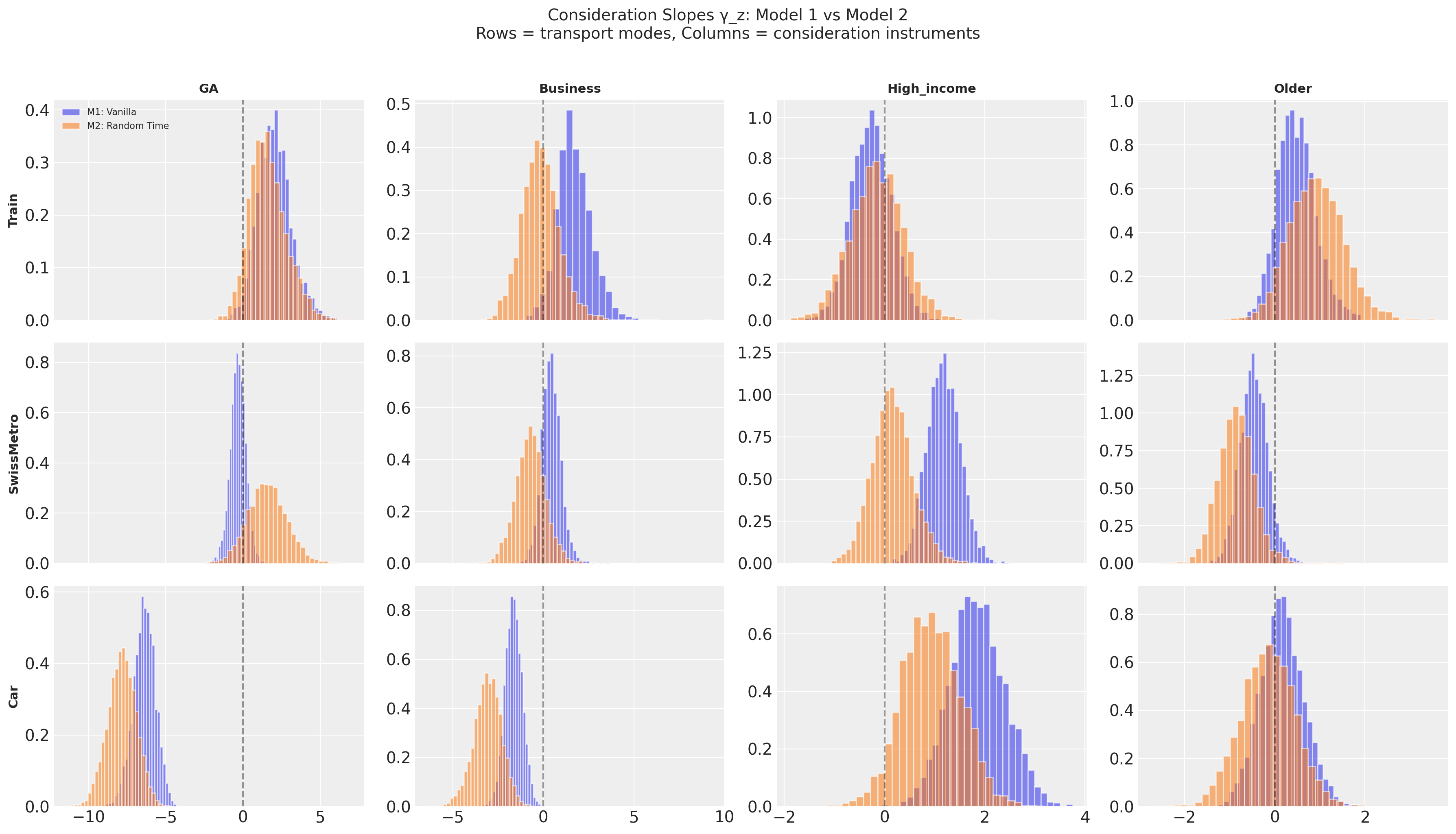
The High_income × Car Sign Flip

The striking result is the potential for sign flips between models. In M1, the posterior is mostly positive: high income increases car consideration. Intuitive enough, since wealthier people are more likely to own cars. In M2, the sign flips allow negative values for high earner consideration of cars.

The explanation is confounding between time sensitivity and income. High-income individuals tend to have a higher value of time. In M1, with fixed time coefficients, the model cannot capture this, so gamma_z[X, High_income] absorbs the effect. High earners appear to consider Car more when they are really responding more strongly to Car’s door-to-door speed advantage.

M2 introduces random coefficients on travel time. Individual-level time sensitivity is now captured by \(\beta^{tt}_n\). The consideration slope is freed to reflect the residual income effect: conditional on time preferences, high-income Swiss travellers are less likely to consider Car, perhaps because they are the urban professionals who hold GA passes and default to rail.

The lesson is plain. Consideration parameters are only identifiable up to the quality of the utility specification. A misspecified utility stage does not just produce wrong utility estimates. It contaminates the consideration story.

Counterfactual: What if Everyone Held a GA Pass?

The consideration set model lets us simulate interventions that widen the streetlamp rather than change what’s underneath it. Here we give every traveller a GA pass, shifting the GA column of Z_tilde to its maximum.

A necessary caveat

This counterfactual is a stress test of the model, not a policy forecast. People who lack a GA pass often have good reasons: they live far from rail, travel infrequently, or prefer driving. GA ownership is endogenous to lifestyle and geography, not randomly assigned. Giving everyone a pass in the model changes where the drunk looks, but cannot change where the keys are.

GA is really a proxy for rail-embeddedness. Extrapolating to universal ownership pushes far beyond the support of the data. Read the results below as “what the model thinks would happen,” not “what would happen.”

The sensitivity of gamma_z to utility-stage specification reinforces this caution. The sign flip on High_income × Car shows that consideration parameters absorb different things depending on what the utility stage captures. A counterfactual built on M1’s estimates would tell a different story than one built on M2’s.

# Counterfactual: universal GA — everyone holds a rail pass
# The GA instrument is the first column (index 0) in Z_tilde[:, :, 0]
# Under the counterfactual, GA = 1 for everyone, so Z_tilde_GA = 1 - mean(GA)
Z_tilde_cf = Z_tilde.copy()
ga_shift = 1.0 - Z_means[0]  # shift from mean-centred to "everyone has GA"
Z_tilde_cf[:, :, 0] = ga_shift  # set GA instrument to counterfactual for all modes

print(f"Baseline GA rate: {Z_means[0]:.1%}")
print("Counterfactual: universal GA (100%)")
print(f"GA Z_tilde shifts from mean 0 to {ga_shift:.3f}")

# Apply intervention using Model 2 (random time)
idata_cf = model_random.apply_intervention(
    new_choice_df=df_sub,
    new_consideration_instruments={
        "Z_tilde": Z_tilde_cf,
        "z_instrument_names": z_names,
    },
)

Sampling: [likelihood]

Baseline GA rate: 15.6%
Counterfactual: universal GA (100%)
GA Z_tilde shifts from mean 0 to 0.844

# Compare market shares: baseline vs counterfactual
# model_random.idata has posterior_predictive from sample_posterior_predictive()
p_baseline = (
    model_random.idata.posterior_predictive["p"].mean(dim=["chain", "draw"]).values
)
p_cf = idata_cf.posterior_predictive["p"].mean(dim=["chain", "draw"]).values

share_baseline = p_baseline.mean(axis=0)
share_cf = p_cf.mean(axis=0)

share_df = pd.DataFrame(
    {
        "Alternative": alt_names,
        "Baseline Share": share_baseline,
        "Counterfactual Share": share_cf,
        "Change": share_cf - share_baseline,
        "% Change": 100 * (share_cf - share_baseline) / share_baseline,
    }
).round(4)

print("Market Share Impact of Universal GA Pass:")
share_df

Market Share Impact of Universal GA Pass:

	Alternative	Baseline Share	Counterfactual Share	Change	% Change
0	Train	0.1342	0.1886	0.0544	40.5264
1	SwissMetro	0.5840	0.8000	0.2160	36.9818
2	Car	0.2818	0.0114	-0.2704	-95.9596

Show code cell source

Hide code cell source

# Visualise the share change
fig, ax = plt.subplots(figsize=(9, 5))
x = np.arange(len(alt_names))
width = 0.35
bars1 = ax.bar(x - width / 2, share_baseline, width, label="Baseline", alpha=0.4)
bars2 = ax.bar(
    x + width / 2,
    share_cf,
    width,
    label="Counterfactual (universal GA)",
    alpha=0.4,
)
ax.set_xticks(x)
ax.set_xticklabels(alt_names)
ax.set_ylabel("Market Share")
ax.set_title(
    "Impact of Universal GA Pass on Market Shares\n"
    "(consideration-stage intervention only)"
)
ax.legend(loc="upper left", bbox_to_anchor=(1.01, 1), borderaxespad=0)

# Add change annotations
for i, (b, cf) in enumerate(zip(share_baseline, share_cf, strict=True)):
    change = cf - b
    ax.annotate(
        f"{change:+.3f}",
        xy=(x[i] + width / 2, cf),
        ha="center",
        va="bottom",
        fontsize=10,
        fontweight="bold",
    )

plt.tight_layout()

/var/folders/__/ng_3_9pn1f11ftyml_qr69vh0000gn/T/ipykernel_79640/2742789636.py:34: UserWarning: The figure layout has changed to tight
  plt.tight_layout()

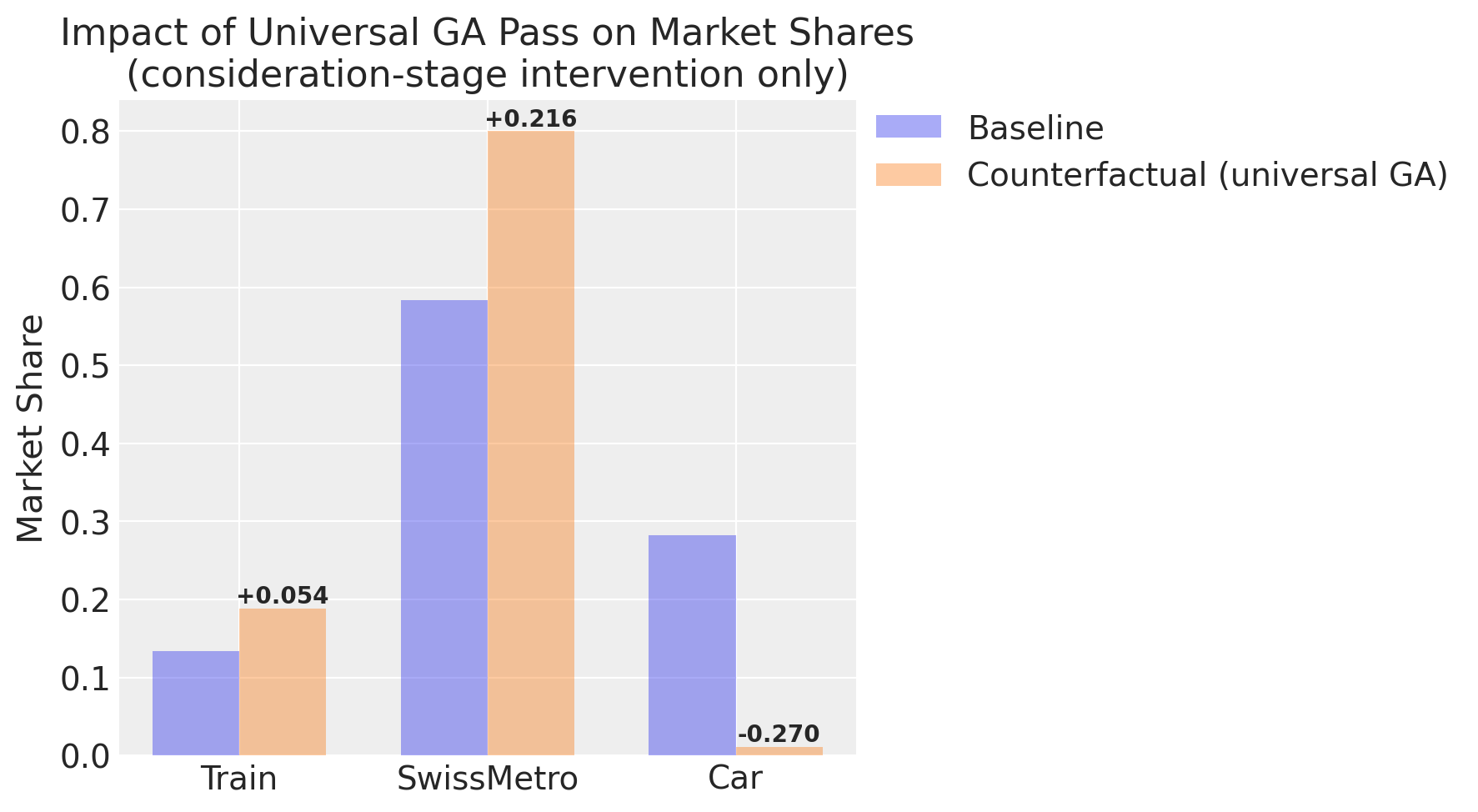
The near-zero car share is implausible. People own cars and use them for reasons unrelated to lacking a rail pass. But the value of the counterfactual is in the mechanism, not the numbers.

In settings where the exclusion restriction is more defensible, this framework quantifies something important. Consider hiring. Race or gender may affect whether a candidate is seen without affecting their productivity conditional on evaluation. A consideration set model applied to hiring data would decompose how much of the outcome is driven by the narrowness of the consideration set versus genuine preference. The counterfactual probe would then quantify the cost of bias at the screening stage, where its effects are most dramatic and most actionable.

The Swiss Metro example clouds the picture because GA plausibly plays two roles: it drives consideration and proxies for utility (rail-embedded lifestyles correlate with rail-favourable preferences). In an ideal application, the screening instruments would be independent of the utility calculation but meaningful for the consideration calculation.

Summary

Consideration dominates the Swiss Metro choice setting. The gamma_z slopes, especially for GA, are large relative to utility parameters. Who notices what matters at least as much as how they evaluate it.

The comparison between models sharpens this conclusion and complicates it. Adding random effects on travel time (Model 2) flips the sign on High_income × Car, showing that consideration parameters absorb whatever the utility stage fails to capture. Both stages need proper specification, and no single model’s consideration estimates should be taken at face value without comparison.

The counterfactual exercise reinforces the point. The universal-GA scenario is deliberately extreme and produces implausible predictions. Its value is not in the numbers but in revealing the model’s structure: how much screening matters, and where the instruments are doing real work versus proxying for unmodeled preference heterogeneity. In domains with cleaner exclusion restrictions, such as hiring, the same framework would produce more credible counterfactuals and more actionable diagnoses.

Consideration is competitive

The simulated hiring counterfactual illustrates a subtler point: consideration is zero-sum. Market shares must sum to one, so when a policy or intervention raises the visibility of some firms it necessarily lowers the relative share of others — even firms whose own screening probabilities barely move. In the network-score counterfactual, Firm B’s consideration probability is nearly unchanged, yet it loses roughly 20% of its baseline share simply because Firms A and C became more visible. Firm B is not the target of the intervention; it is collateral.

This has a direct managerial implication. A firm should monitor the consideration instruments of its competitors, not just its own. A rival that improves its network reach, or benefits from a broad platform or subscription that embeds it in customers’ routines, can erode your share without your product or service changing at all. Consideration is not a fixed attribute of an alternative — it is shaped by the entire competitive landscape and by whatever mechanisms route customers toward or away from alternatives in the first place.

The ConsiderationSetMixedLogit class extends the existing MixedLogit with a consideration stage, supports multiple instruments per alternative, and provides apply_intervention for counterfactual analysis.

%load_ext watermark
%watermark -n -u -v -iv -w -p pymc_marketing

Last updated: Sun Apr 19 2026

Python implementation: CPython
Python version       : 3.12.12
IPython version      : 9.8.0

pymc_marketing: 0.19.0

matplotlib    : 3.10.8
pymc          : 5.28.2
pandas        : 2.3.3
pymc_marketing: 0.19.0
numpy         : 2.3.5
arviz         : 0.23.0

Watermark: 2.5.0